Validating customer matching in uplift analysis
Introduction
What is matching
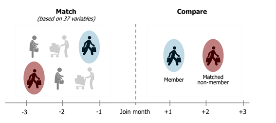
Statistical matching is the process where we pair up responses in the treatment group with their respective doppelganger from the untreated group.
Once matched these groups can be compared similar to a DoE treatment group.
Problem statement
Often during performance analytics we have to use statistical matching to construct a control group post program launch.
In this case we may want to validate the quality of the matching.
I propose here a method for comparing the matching between treated and untreated to matches in the treated group only.
The purpose of the matching is a replacement for treatment groups, so that we believe that between the 2 groups we have now controlled for confounding in atleast the extent that the customers were matched to one another.
To test if the matching is predictive then; we could bootstrap the uplift (the difference in spend between 2 groups) within only the control (matched to) and treated (joined and matched) respectively. This would require us to do matching within these 2 cohorts again, since we need to compare a person to his/her doppelganger.
Null hypothesis
If our matching process has indeed controlled for lurker effects with respect to the measured response then matching within the treatment group only will reveal no real lift in the response of interest.
By comparison the matched groups between those treated or not will reveal comparitively greater lift when bootstrapped.
Example case
For our example we have MFA output extracting components out of a payment behavior dataset:
MFA_output_2014_01_01 %>% glimpse## Observations: 456,366
## Variables: 40
## $ customer_no <int> 13, 51, 82, 98, 139, 170, 1...
## $ vitality <int> 0, 0, 0, 0, 0, 0, 0, 0, 0, ...
## $ `spend_month_spend_sum_2013-10-01` <dbl> 12281.10, 0.00, 1585.58, 53...
## $ `spend_month_spend_sum_2013-11-01` <dbl> 12137.86, 0.00, 0.00, 8136....
## $ `spend_month_spend_sum_2013-12-01` <dbl> 12769.57, 541.62, 5609.84, ...
## $ `1` <dbl> 2.206990e+00, -9.920552e-01...
## $ `2` <dbl> 0.34242884, -2.20506687, -0...
## $ `3` <dbl> 0.34804986, -1.95304588, 0....
## $ `4` <dbl> -1.696023886, -1.385098798,...
## $ `5` <dbl> -0.30175202, -0.47332798, -...
## $ `6` <dbl> -0.42201805, 1.30042399, -0...
## $ `7` <dbl> -0.77934720, 0.30207369, 0....
## $ `8` <dbl> -0.68034669, 0.07018387, 0....
## $ `9` <dbl> -0.27725997, -0.16822390, -...
## $ `10` <dbl> 0.01296691, 0.16549627, -0....
## $ `11` <dbl> 0.130646590, -0.144442768, ...
## $ `12` <dbl> 0.11638400, -1.51874464, -0...
## $ `13` <dbl> 0.088020420, -0.373939500, ...
## $ `14` <dbl> -0.22521735, 0.13691562, -0...
## $ `15` <dbl> 0.088687700, 0.593443274, 0...
## $ `16` <dbl> 0.52900438, -0.22733655, -0...
## $ `17` <dbl> -0.03321893, -0.70535188, -...
## $ `18` <dbl> 0.06344598, 1.07738851, 1.3...
## $ `19` <dbl> 0.04313334, -0.11892780, -0...
## $ `20` <dbl> 0.31355059, 0.02262493, -0....
## $ `21` <dbl> 0.515642127, 0.033112011, -...
## $ `22` <dbl> 0.46893878, 0.91978096, 0.7...
## $ `23` <dbl> -1.16564871, 0.29106354, -0...
## $ `24` <dbl> -0.37090531, -0.14419326, -...
## $ `25` <dbl> -0.64744784, -0.23397443, -...
## $ `26` <dbl> -0.467301732, -0.251150460,...
## $ `27` <dbl> -0.19584238, -0.19355691, -...
## $ `28` <dbl> 0.33062267, 0.25182759, 0.4...
## $ `29` <dbl> -0.03982754, 0.11362521, 0....
## $ `30` <dbl> -0.38005037, 0.13911337, -0...
## $ `31` <dbl> 0.22410782, -0.78493345, -0...
## $ `32` <dbl> 0.06572623, -0.01481643, -0...
## $ `33` <dbl> 0.472780487, 0.082725681, 0...
## $ `34` <dbl> 0.12830024, -0.35510797, 0....
## $ `35` <dbl> -0.29165777, -0.01369455, -...This data summarises customer spend and demographics data through 35 MFA principal components.
Genetic matching was performed on this data to produce our treatment groups.
Initial validation
As an immediate check it’s a good idea to visualize the different metrics for your matched groups:
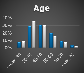
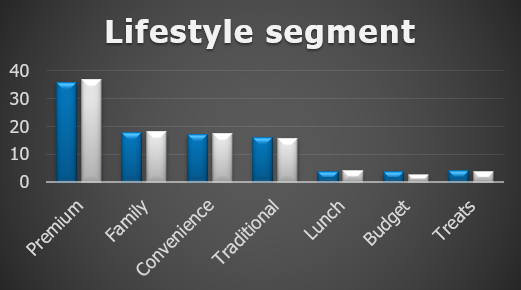
Summary metrics
For validation we want to investigate the ATV and ATF.
ATV is the average transavtion value.
ATF is the average number of transactions.
Careful; when matching one to many the join onto the spend data will created weighted duplicates. Make sure how you calculate ATV and ATF. You want to weight and aggregate the spend and matched spend before you start taking averages over the grouping variables of interest
Visualization
When applying genetic matching to a single cohort month 2014_01 our analysis reveals the following ATV:
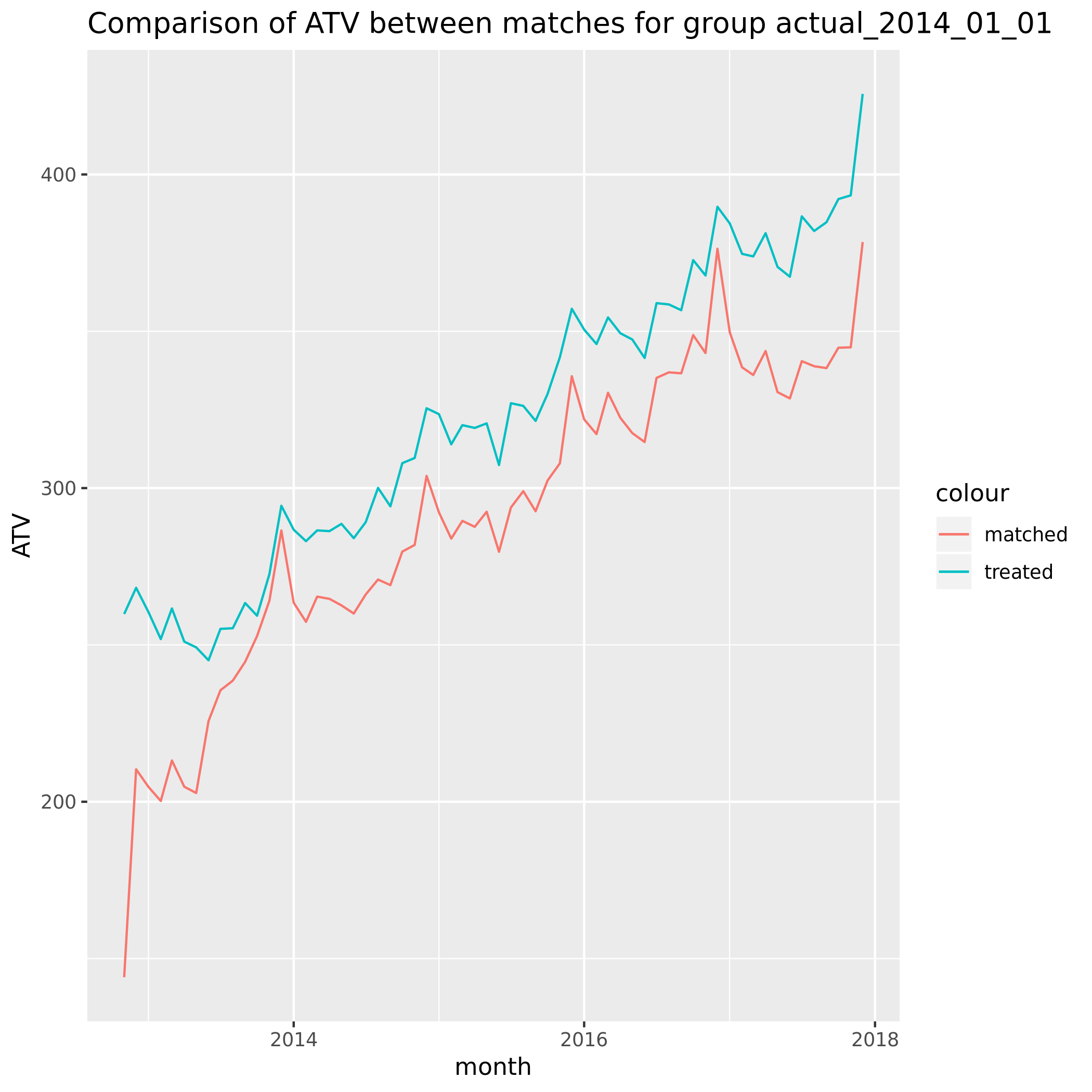
The matching was performed on the 3 months prior to Jan 2014. For this cohort at least something concerning is that the matches don’t appear similar in aggregate for the months before that.
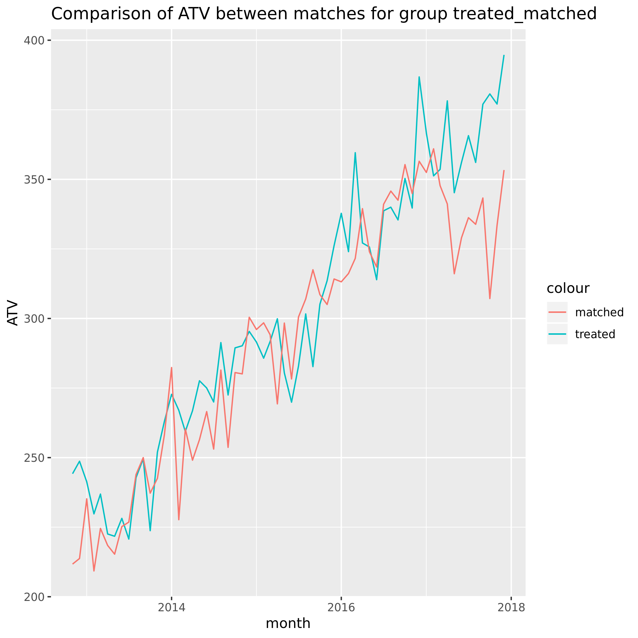
For a benchmark we can perform matching once again. This time we perform the matching only within the treatment group. We do this by assigning treated randomly accross the customers in this group and matching based on this randomly assigned binary outcome.
This is what it looked like:
Initial conclusions
This is somewhat reassuring. The matching pre-period needs to be investigated further but we can tell that randomizing treatment assignment did in fact lead to a balanced response of ATV in the 2 groups.
If there were untracked effects we wouldn’t expect these to be similar within the treatment group.
Bootstrapping
What we also want to do is bootstrap the ATV and ATF statistics for our match groups.
This is simple to execute once you have your match and spend data in the correct format.
Define bootstrapping function:
library(boot)

bootstrap_stats <- function(match_spend_data, bootstrap_size = 1000, group = "group"){

  get_mean_var <- function(data, indices){
  d <- data[indices,]

  mean_ATV <- mean(d$ATV,na.rm=T)
  mean_ATV_matched <- mean(d$ATV_matched ,na.rm=T)
  var_ATV <- var(d$ATV,na.rm=T)
  var_ATV_matched <- var(d$ATV_matched ,na.rm=T)
  mean_transactions <- mean(d$nr_transactions,na.rm=T)
  mean_transactions_matched <- mean(d$nr_transactions_matched,na.rm=T)
  var_transactions <- var(d$nr_transactions,na.rm=T)
  var_transactions_matched <- var(d$nr_transactions_matched,na.rm=T)

  return(c(mean_ATV,mean_ATV_matched,var_ATV,var_ATV_matched,mean_transactions,mean_transactions_matched,var_transactions,var_transactions_matched))
  # return(c(mean_ATV = mean_ATV,var_ATV = var_ATV,mean_ATV_matched = mean_ATV_matched,var_ATV_matched = var_ATV_matched))
}

boot_data <-
  match_spend_data %>%
  group_by(customer_no) %>%
  summarise(ATV = mean(ATV, na.rm = T),
            ATV_matched = mean(ATV_matched , na.rm = T),
            nr_transactions = mean(nr_transactions,na.rm=T),
            nr_transactions_matched = mean(nr_transactions_matched,na.rm=T)
            )

results <- boot(boot_data, statistic=get_mean_var, R=bootstrap_size)

bootsrap_results <-
  tibble(
    variable = c("mean_ATV","mean_ATV_matched","var_ATV","var_ATV_matched","mean_transactions","mean_transactions_matched","var_transactions","var_transactions_matched"),
    bootrap_value = results$t0,
    sd = results$t %>% apply(MARGIN = 2,sd),
    lower = bootrap_value - 1.5*sd,
    upper = bootrap_value + 1.5*sd
  ) %>%
  mutate(group = group)

bootsrap_results
}
Apply it:
match_design <-
tibble(group = c("actual_2014_01_01","treated_matched","control_matched"),
spend_data = list(spend_table), match_data = list(readRDS("../Data/cohort_2014_01_01_matches.rds"),prepare_matches_treated,
prepare_matches_control))
match_design <-
match_design %>%
mutate(match_comparison_results = pmap(list(spend_data,match_data,group),~compare_matches(..2,..1,..3)))
match_design <-
match_design %>%
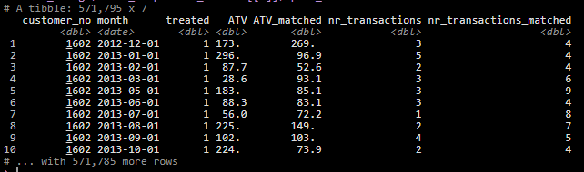
mutate(bootrap_statistics = map2(.x = match_comparison_results, .y = group,~bootstrap_stats(match_spend_data = .x$spend_table,bootstrap_size = 1000, group = .y)))The data once matched looked like this:
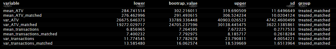
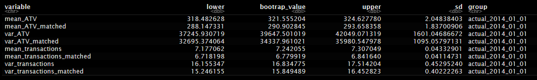
Bootstrapped actuals:
Bootstrapped treated: