
Test multiple sklearn models with LIME
In this blog I load the toy dataset for detecting breast cancer. Often before you can fine tune and productionize any model you will have to play with and test a wide range of models.
Luckily we have frameworks like scikit_learn and caret to train many different models! Prepare yourself

import numpy
import pandas
import matplotlib.pyplot as plt
from sklearn import model_selection
from sklearn.linear_model import LogisticRegression
from sklearn.tree import DecisionTreeClassifier
from sklearn.neighbors import KNeighborsClassifier
from sklearn.discriminant_analysis import LinearDiscriminantAnalysis
from sklearn.naive_bayes import GaussianNB
from sklearn.svm import SVC
from sklearn.ensemble import GradientBoostingClassifier
from sklearn.ensemble import RandomForestClassifier
from sklearn.datasets import load_breast_cancer
## Load the data
data, labels = load_breast_cancer(return_X_y=True)
data[1:20,5:9]
array([[ 0.07864,  0.0869 ,  0.07017,  0.1812 ],
       [ 0.1599 ,  0.1974 ,  0.1279 ,  0.2069 ],
       [ 0.2839 ,  0.2414 ,  0.1052 ,  0.2597 ],
       [ 0.1328 ,  0.198  ,  0.1043 ,  0.1809 ],
       [ 0.17   ,  0.1578 ,  0.08089,  0.2087 ],
       [ 0.109  ,  0.1127 ,  0.074  ,  0.1794 ],
       [ 0.1645 ,  0.09366,  0.05985,  0.2196 ],
       [ 0.1932 ,  0.1859 ,  0.09353,  0.235  ],
       [ 0.2396 ,  0.2273 ,  0.08543,  0.203  ],
       [ 0.06669,  0.03299,  0.03323,  0.1528 ],
       [ 0.1292 ,  0.09954,  0.06606,  0.1842 ],
       [ 0.2458 ,  0.2065 ,  0.1118 ,  0.2397 ],
       [ 0.1002 ,  0.09938,  0.05364,  0.1847 ],
       [ 0.2293 ,  0.2128 ,  0.08025,  0.2069 ],
       [ 0.1595 ,  0.1639 ,  0.07364,  0.2303 ],
       [ 0.072  ,  0.07395,  0.05259,  0.1586 ],
       [ 0.2022 ,  0.1722 ,  0.1028 ,  0.2164 ],
       [ 0.1027 ,  0.1479 ,  0.09498,  0.1582 ],
       [ 0.08129,  0.06664,  0.04781,  0.1885 ]])
type(data)
numpy.ndarray
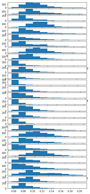
We have 569 observations in this case study and we have recorded 30 different markers to help us predict breast cancer:
data.shape
(569, 30)
In this case we have loaded a nice and clean toy dataset. However, it is always a good idea to make sure all of your variables are balanced and scaled.
Dealing with class imbalances and deep categorical levels is beyond the scope of this blog.
Here is an example of how you could look at your variables:
plots_data = [i for i in data.T]

for i in range(1,len(plots_data)):
    plt.subplot(len(plots_data),1 , i)
    plt.hist(plots_data[i])

F = plt.gcf()
F.set_figheight(15)
plt.show()
labels[1:100]
array([0, 0, 0, 0, 0, 0, 0, 0, 0, 0, 0, 0, 0, 0, 0, 0, 0, 0, 1, 1, 1, 0, 0,
       0, 0, 0, 0, 0, 0, 0, 0, 0, 0, 0, 0, 0, 1, 0, 0, 0, 0, 0, 0, 0, 0, 1,
       0, 1, 1, 1, 1, 1, 0, 0, 1, 0, 0, 1, 1, 1, 1, 0, 1, 0, 0, 1, 1, 1, 1,
       0, 1, 0, 0, 1, 0, 1, 0, 0, 1, 1, 1, 0, 0, 1, 0, 0, 0, 1, 1, 1, 0, 1,
       1, 0, 0, 1, 1, 1, 0])
Define model pipeline
Now we define a list of models we would like to test on this data:
X = data
Y = labels
# prepare configuration for cross validation test harness
seed = 8020
# prepare models
models = []
models.append(('LR', LogisticRegression()))
models.append(('LDA', LinearDiscriminantAnalysis()))
models.append(('KNN', KNeighborsClassifier()))
models.append(('CART', DecisionTreeClassifier()))
models.append(('NB', GaussianNB()))
models.append(('SVM', SVC()))
models.append(('RF', RandomForestClassifier()))
models.append(('GBM', GradientBoostingClassifier()))
models
[('LR',
  LogisticRegression(C=1.0, class_weight=None, dual=False, fit_intercept=True,
            intercept_scaling=1, max_iter=100, multi_class='ovr', n_jobs=1,
            penalty='l2', random_state=None, solver='liblinear', tol=0.0001,
            verbose=0, warm_start=False)),
 ('LDA',
  LinearDiscriminantAnalysis(n_components=None, priors=None, shrinkage=None,
                solver='svd', store_covariance=False, tol=0.0001)),
 ('KNN',
  KNeighborsClassifier(algorithm='auto', leaf_size=30, metric='minkowski',
             metric_params=None, n_jobs=1, n_neighbors=5, p=2,
             weights='uniform')),
 ('CART',
  DecisionTreeClassifier(class_weight=None, criterion='gini', max_depth=None,
              max_features=None, max_leaf_nodes=None,
              min_impurity_decrease=0.0, min_impurity_split=None,
              min_samples_leaf=1, min_samples_split=2,
              min_weight_fraction_leaf=0.0, presort=False, random_state=None,
              splitter='best')),
 ('NB', GaussianNB(priors=None)),
 ('SVM', SVC(C=1.0, cache_size=200, class_weight=None, coef0=0.0,
    decision_function_shape='ovr', degree=3, gamma='auto', kernel='rbf',
    max_iter=-1, probability=False, random_state=None, shrinking=True,
    tol=0.001, verbose=False)),
 ('RF',
  RandomForestClassifier(bootstrap=True, class_weight=None, criterion='gini',
              max_depth=None, max_features='auto', max_leaf_nodes=None,
              min_impurity_decrease=0.0, min_impurity_split=None,
              min_samples_leaf=1, min_samples_split=2,
              min_weight_fraction_leaf=0.0, n_estimators=10, n_jobs=1,
              oob_score=False, random_state=None, verbose=0,
              warm_start=False)),
 ('GBM', GradientBoostingClassifier(criterion='friedman_mse', init=None,
                learning_rate=0.1, loss='deviance', max_depth=3,
                max_features=None, max_leaf_nodes=None,
                min_impurity_decrease=0.0, min_impurity_split=None,
                min_samples_leaf=1, min_samples_split=2,
                min_weight_fraction_leaf=0.0, n_estimators=100,
                presort='auto', random_state=None, subsample=1.0, verbose=0,
                warm_start=False))]
Now that we have a list of tuples whith a model name and a model object to be trained we can loop over these pairs of tuples and call their fit and crossvalidation methods:
# evaluate each model in turn
results = []
names = []
scoring = 'accuracy'
for name, model in models:
	kfold = model_selection.KFold(n_splits=4, random_state=seed)
	cv_results = model_selection.cross_val_score(model, X, Y, cv=kfold, scoring=scoring)
	results.append(cv_results)
	names.append(name)
	msg = "%s: %f (%f)" % (name, cv_results.mean(), cv_results.std())
	model.fit(X=X,y=Y)
	print(msg)
LR: 0.947319 (0.015929)
LDA: 0.956134 (0.028991)
KNN: 0.919273 (0.039560)
CART: 0.896373 (0.044996)
NB: 0.936829 (0.034158)
SVM: 0.627770 (0.144022)
RF: 0.952613 (0.021670)
GBM: 0.952637 (0.032907)
Notice that the cross_val_score method will not return you a fitted object since it is evaluating the model over each fold. So we also train each model on all the data for use later.
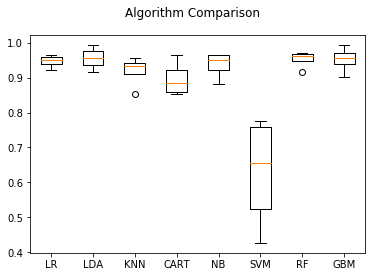
Now that we have reported the crossvalidated scores we can also plot them to see how consistent each model’s accuracy was over the different folds:
# boxplot algorithm comparison
fig = plt.figure()
fig.suptitle('Algorithm Comparison')
ax = fig.add_subplot(111)
plt.boxplot(results)
ax.set_xticklabels(names)
plt.show()
Use LIME to explain breast cancer prediction
import lime
import lime.lime_tabular
from __future__ import print_function
Lime uses defined explainers to produce reports. To use these explainers we need to provide them with: - data going into the model - names of the variables - specify categorical variables - specify the outcome (if categorical) - give a function that will make predictions
We can make lamda functions that take the input and make a prediction using the model objects built in methods
model_objects = [i[1] for i in models]
predict_fn_logreg = lambda x: model_objects[0].predict_proba(x).astype(float)
predict_fn_svc = lambda x: model_objects[5].predict_proba(x).astype(float)
predict_fn_rf = lambda x: model_objects[6].predict_proba(x).astype(float)
predict_fn_gbm = lambda x: model_objects[7].predict_proba(x).astype(float)
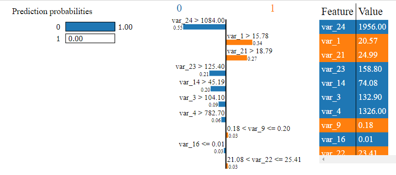
Explain logistic regression
explainer = lime.lime_tabular.LimeTabularExplainer(X,feature_names=['var_'+str(i) for i in range(1,X.shape[1]+1)],categorical_names=['No','Yes'])
The reports will explain which variables suggested what outcome. In the logistic case we see that the model looks somewhat unsure about some of these signals even though overall it is very confident:
%%capture
observation = 1
exp = explainer.explain_instance(X[observation],predict_fn=predict_fn_logreg)
exp.show_in_notebook()
    <script>
    var top_div = d3.select('#top_divCFB8TSK64189N6A').classed('lime top_div', true);

        var pp_div = top_div.append('div')
                            .classed('lime predict_proba', true);
        var pp_svg = pp_div.append('svg').style('width', '100%');
        var pp = new lime.PredictProba(pp_svg, ["0", "1"], [0.9999999796028671, 2.039713284887131e-08]);


    var exp_div;
        var exp = new lime.Explanation(["0", "1"]);

            exp_div = top_div.append('div').classed('lime explanation', true);
            exp.show([["var_24 > 1084.00", -0.5522436379485604], ["var_1 > 15.78", 0.34089875250006835], ["var_21 > 18.79", 0.27241545277342066], ["var_23 > 125.40", -0.21374112919123914], ["var_14 > 45.19", -0.1973896374910405], ["var_3 > 104.10", -0.09457934839642751], ["var_4 > 782.70", -0.05875935288375921], ["0.18 < var_9 <= 0.20", 0.028114709663375852], ["var_16 <= 0.01", -0.025900312503506027], ["21.08 < var_22 <= 25.41", 0.025424488183932236]], 1, exp_div);

    var raw_div = top_div.append('div');
        exp.show_raw_tabular([["var_24", "1956.00", -0.5522436379485604], ["var_1", "20.57", 0.34089875250006835], ["var_21", "24.99", 0.27241545277342066], ["var_23", "158.80", -0.21374112919123914], ["var_14", "74.08", -0.1973896374910405], ["var_3", "132.90", -0.09457934839642751], ["var_4", "1326.00", -0.05875935288375921], ["var_9", "0.18", 0.028114709663375852], ["var_16", "0.01", -0.025900312503506027], ["var_22", "23.41", 0.025424488183932236]], 1, raw_div);

    </script>
    </body></html>
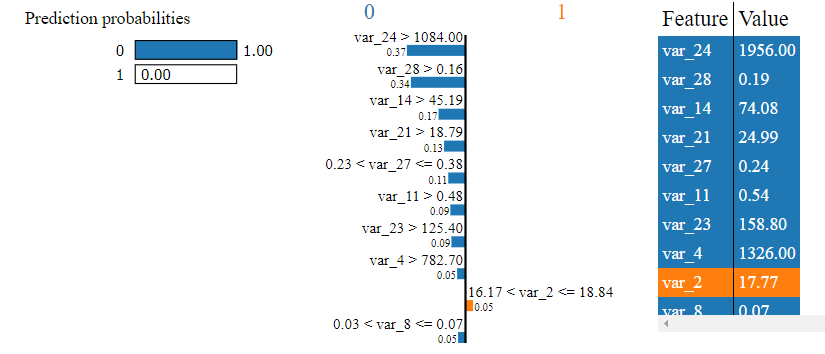
Explain gradient boosted machine
%%capture
exp = explainer.explain_instance(X[observation],predict_fn=predict_fn_gbm)
exp.show_in_notebook()
    <script>
    var top_div = d3.select('#top_divZ8PE4P100D1W9IC').classed('lime top_div', true);

        var pp_div = top_div.append('div')
                            .classed('lime predict_proba', true);
        var pp_svg = pp_div.append('svg').style('width', '100%');
        var pp = new lime.PredictProba(pp_svg, ["0", "1"], [0.998513484638384, 0.0014865153616160618]);


    var exp_div;
        var exp = new lime.Explanation(["0", "1"]);

            exp_div = top_div.append('div').classed('lime explanation', true);
            exp.show([["var_24 > 1084.00", -0.36730312198081294], ["var_28 > 0.16", -0.3423587715973614], ["var_14 > 45.19", -0.16883543759143507], ["var_21 > 18.79", -0.1342287961256812], ["0.23 < var_27 <= 0.38", -0.1081794378458047], ["var_11 > 0.48", -0.0946891446826724], ["var_23 > 125.40", -0.08841597688343487], ["var_4 > 782.70", -0.0525452616340418], ["16.17 < var_2 <= 18.84", 0.04739117251897969], ["0.03 < var_8 <= 0.07", -0.04667251216709414]], 1, exp_div);

    var raw_div = top_div.append('div');
        exp.show_raw_tabular([["var_24", "1956.00", -0.36730312198081294], ["var_28", "0.19", -0.3423587715973614], ["var_14", "74.08", -0.16883543759143507], ["var_21", "24.99", -0.1342287961256812], ["var_27", "0.24", -0.1081794378458047], ["var_11", "0.54", -0.0946891446826724], ["var_23", "158.80", -0.08841597688343487], ["var_4", "1326.00", -0.0525452616340418], ["var_2", "17.77", 0.04739117251897969], ["var_8", "0.07", -0.04667251216709414]], 1, raw_div);

    </script>
    </body></html>
Explain random forest
%%capture
exp = explainer.explain_instance(X[observation],predict_fn=predict_fn_rf)
exp.show_in_notebook()
    <script>
    var top_div = d3.select('#top_divNBG3I2J8YFBS8XE').classed('lime top_div', true);

        var pp_div = top_div.append('div')
                            .classed('lime predict_proba', true);
        var pp_svg = pp_div.append('svg').style('width', '100%');
        var pp = new lime.PredictProba(pp_svg, ["0", "1"], [1.0, 0.0]);


    var exp_div;
        var exp = new lime.Explanation(["0", "1"]);

            exp_div = top_div.append('div').classed('lime explanation', true);
            exp.show([["var_28 > 0.16", -0.16422274051889757], ["var_23 > 125.40", -0.1460412598938762], ["var_11 > 0.48", -0.11794644087970245], ["var_24 > 1084.00", -0.09632721244740866], ["var_21 > 18.79", -0.09340363310604781], ["var_14 > 45.19", -0.07788668325377436], ["var_3 > 104.10", -0.05074094108145428], ["0.23 < var_27 <= 0.38", -0.04457243654253311], ["var_4 > 782.70", -0.032670824142992834], ["21.08 < var_22 <= 25.41", 0.026368543351076034]], 1, exp_div);

    var raw_div = top_div.append('div');
        exp.show_raw_tabular([["var_28", "0.19", -0.16422274051889757], ["var_23", "158.80", -0.1460412598938762], ["var_11", "0.54", -0.11794644087970245], ["var_24", "1956.00", -0.09632721244740866], ["var_21", "24.99", -0.09340363310604781], ["var_14", "74.08", -0.07788668325377436], ["var_3", "132.90", -0.05074094108145428], ["var_27", "0.24", -0.04457243654253311], ["var_4", "1326.00", -0.032670824142992834], ["var_22", "23.41", 0.026368543351076034]], 1, raw_div);

    </script>
    </body></html>
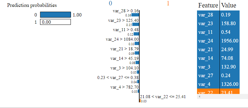
We can see more consistency between the random forest and gradient boosted machine but even here different variables are used to arrive at a prediction. Perhaps we could boost some of these models to improve performance or tune them further.