
Predict house prices - deep learning, keras
Overview
In this notebook I fool around with some fast prototype models for predicting house prices using deep neural nets!

First I will do some LSTM modelling for the house price movement using tidy backtested crossvalidation.
Next I use tidy crossvalidated dense feed forward networks to predict the price of a property based on the properties descriptions!
Coming soon; I will use the LSTM model to produce a 1 month forecast and feed this as a dimension to the inference model during predictions of houses for which we believe we have the descriptive data now but we will only sell the property in a months time. I will compare the errors by holding out the last few months of data to test the combined accuracy accounting for price movement.
Naive model (no time index)
As a little introduction we can cover the example in the book
For our first model we will be using the boston housing data from 1970. This data collected features of the sale but had no time index - probably because the data was only collected over 1970; possibly with some cencoring.
With no time index in the data we can think of the tensors as being 1D tensors since the samples have n features on only 1 axis.
With this model we cannot really predict into the future so our predictions are only valid for predicting house prices right now (1970).
Load the data
dataset <- dataset_boston_housing()
c(c(train_data, train_targets), c(test_data, test_targets)) %<-% dataset
The training data we load here is already in a matrix format for us:
train_data %>% head## [,1] [,2] [,3] [,4] [,5] [,6] [,7] [,8] [,9] [,10] [,11]
## [1,] 1.23247 0.0 8.14 0 0.538 6.142 91.7 3.9769 4 307 21.0
## [2,] 0.02177 82.5 2.03 0 0.415 7.610 15.7 6.2700 2 348 14.7
## [3,] 4.89822 0.0 18.10 0 0.631 4.970 100.0 1.3325 24 666 20.2
## [4,] 0.03961 0.0 5.19 0 0.515 6.037 34.5 5.9853 5 224 20.2
## [5,] 3.69311 0.0 18.10 0 0.713 6.376 88.4 2.5671 24 666 20.2
## [6,] 0.28392 0.0 7.38 0 0.493 5.708 74.3 4.7211 5 287 19.6
## [,12] [,13]
## [1,] 396.90 18.72
## [2,] 395.38 3.11
## [3,] 375.52 3.26
## [4,] 396.90 8.01
## [5,] 391.43 14.65
## [6,] 391.13 11.74We have 13 features/dimensions of collected data for each sample that we can use to predict the house price:
train_targets %>% head## [1] 15.2 42.3 50.0 21.1 17.7 18.5Scale the variables
mean <- apply(train_data, 2, mean)
std <- apply(train_data, 2, sd)
train_data <- scale(train_data, center = mean, scale = std)
test_data <- scale(test_data, center = mean, scale = std)
Define the model
We can start by defining the model. Since we will be using cross-validation we define a function that constructs the model. We do this because we need to construct and train a model on each fold so we can gauge the performance accross the different folds as we fine tune our model:
Function that constructs a model
Note that I am assuming the data input is a resample object… That’s because I will be creating a tidy crossvalidation and so the objects in my table will be resamples…
I am also assuming the outcome is called ‘target’, but this can be generalised using enquo
define_compile_train_predict <- function(train,test,epochs = 100,shuffle = TRUE,...){

train_X <- train %>% as_tibble() %>% select(-target) %>% as.matrix()
test_X <- test %>% as_tibble() %>% select(-target) %>% as.matrix()
train_y <- train %>% as_tibble() %>%  select(target) %>% as.matrix()
test_y <- test %>% as_tibble() %>%  select(target) %>% as.matrix()

#define
base_model <-
keras_model_sequential() %>%
layer_dense(units = 64, activation = 'relu', input_shape = c(13)) %>% # 1 axis and nr features = number columns
layer_batch_normalization() %>%
# layer_dropout(rate = 0.2) %>%
layer_dense(units = 64, activation ='relu') %>%
# layer_dense(units = 25, activation ='relu') %>%
layer_dense(units = 1)

#compile
base_model %>% compile(
  loss='mse',
  optimizer='rmsprop',
    # optimizer='adam',
  metrics = c('mae')
)

#train
history <- base_model %>%
  keras::fit(train_X,
             train_y,
             epochs=epochs,
             shuffle=shuffle,
             validation_data= list(test_X, test_y),
                verbose = 0
             )

#predict
predictions <-
    base_model %>%
    keras::predict_on_batch(x = train_X)

results <-
base_model %>%
keras::evaluate(test_X, test_y, verbose = 0)

plot_outp <-
    history %>% plot

return(list(predictions = predictions, loss = results$loss, mae = results$mean_absolute_error, plot_outp = plot_outp,base_model=base_model,history = history))

}
In the example in the book they use a for loop to set up the different folds and then apply the training and validation inside these loops. Since R has a lot of this already solved in tidy packages I am just going to leverage them and stay inside of a tidy format so we can keep all the intermediate results and visualize the outputs all in one go
Construct tidy cross-validation
To do this we first setup a nice tibble using the modelr package:
tidy_cross_val <-
    train_data %>%
    as_tibble() %>%
    bind_cols(target = train_targets) %>%
    modelr::crossv_kfold(k = 5) %>%
    rename(fold = .id) %>%
    select(fold,everything())

tidy_cross_val
## # A tibble: 5 x 3
## fold train test
## <chr> <list> <list>
## 1 1 <S3: resample> <S3: resample>
## 2 2 <S3: resample> <S3: resample>
## 3 3 <S3: resample> <S3: resample>
## 4 4 <S3: resample> <S3: resample>
## 5 5 <S3: resample> <S3: resample>Now we can build the models and also compile them, after that we just pluck out the stuff we stored in our function:
# tidy_cross_val$model_output %>% map_dbl(pluck,"mae")
tidy_cross_val <-
tidy_cross_val %>%
mutate(model_output = pmap(list(train = train,test = test), define_compile_train_predict,epochs = 200)) %>%
mutate(mae = model_output %>% map_dbl(pluck,"mae")) %>%
mutate(plot_outp = model_output %>% map(pluck,"plot_outp")) %>%
mutate(loss = model_output %>% map_dbl(pluck,"loss")) %>%
mutate(predictions = model_output %>% map(pluck,"predictions")) %>%
select(everything(),model_output)

tidy_cross_val
## # A tibble: 5 x 8
## fold train test model_output mae plot_outp loss predictions
## <chr> <list> <list> <list> <dbl> <list> <dbl> <list>
## 1 1 <S3: res~ <S3: re~ <list [6]> 2.41 <S3: gg> 10.5 <dbl [323 x~
## 2 2 <S3: res~ <S3: re~ <list [6]> 2.17 <S3: gg> 12.6 <dbl [323 x~
## 3 3 <S3: res~ <S3: re~ <list [6]> 2.24 <S3: gg> 8.56 <dbl [323 x~
## 4 4 <S3: res~ <S3: re~ <list [6]> 2.74 <S3: gg> 13.9 <dbl [323 x~
## 5 5 <S3: res~ <S3: re~ <list [6]> 2.55 <S3: gg> 10.9 <dbl [324 x~By mapping the deeplearning model over all these folds of data we store our results directly into this table. That means we can do interesting things like plot them altogether:
tidy_cross_val %>%
  ggplot(aes(x=fold,y=mae, fill = fold))+
  geom_bar(stat="identity")+
  ggtitle("The k-fold accuracy of the deep neural net",subtitle = "Not yet scaled back...")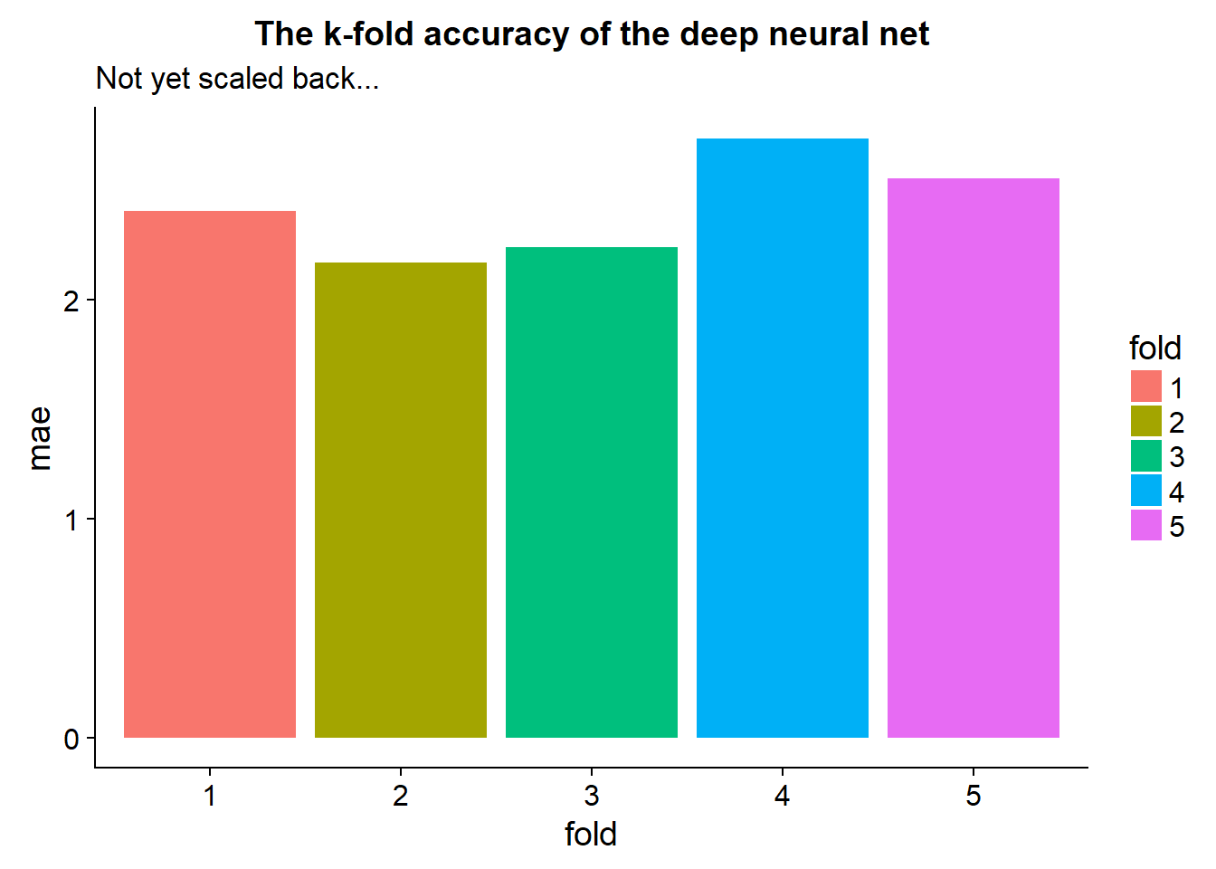
This gives us a good idea of our certainty in the model.
From our tidy cross-validation output we may notice some extreme values for folds in terms of high mae or loss… These should be treated appropriately
Let’s take a closer look at the max mae fold:
tidy_cross_val %>%
filter(.$mae == max(.$mae)) %>%
pull(plot_outp)
## [[1]]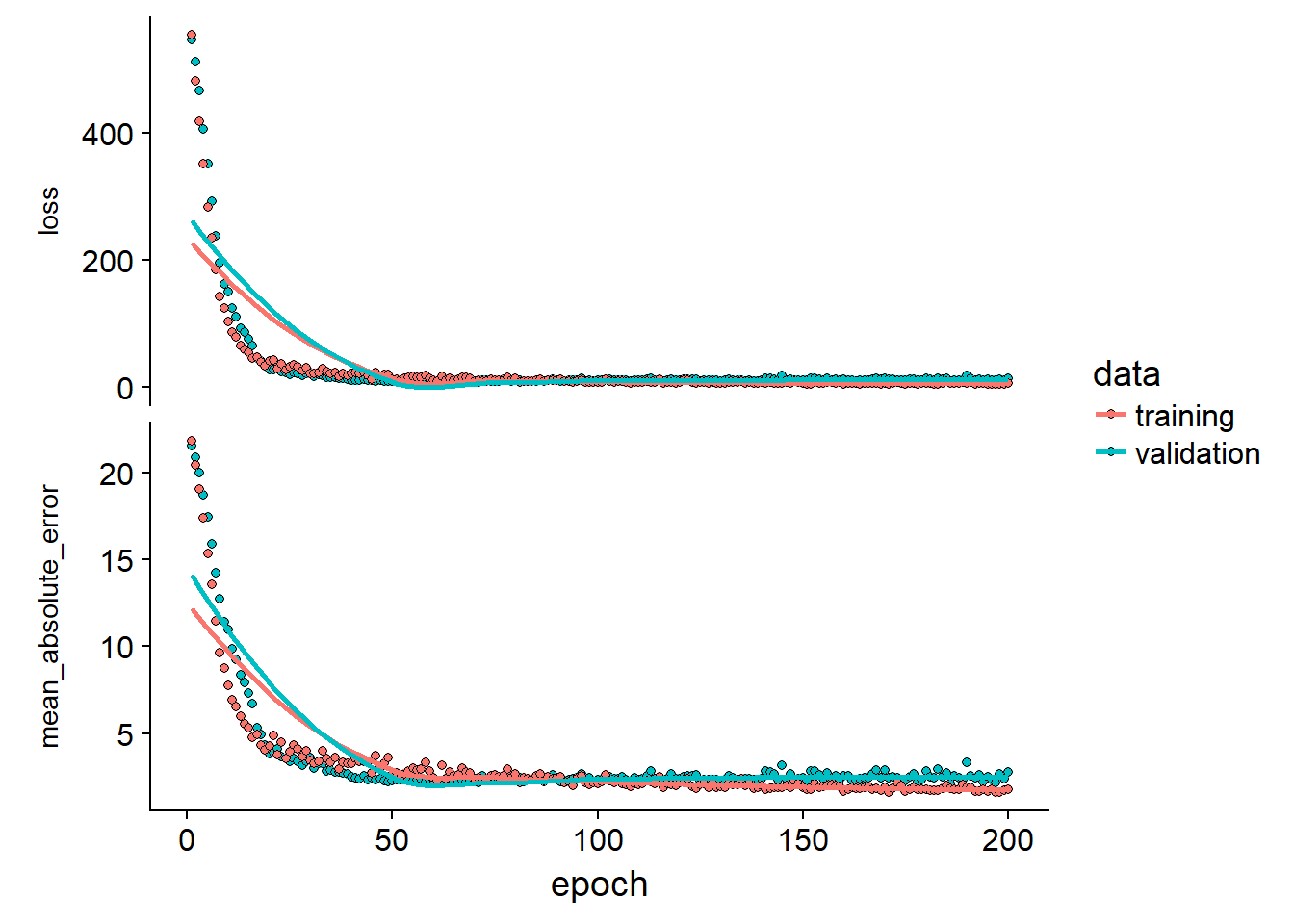
We can look at some extreme folds to see if the validation and training loss diverges which should indicate over-fitting. In this case the model seems to fit great
Measuring over-fit using k-folds crossvalidation
We can visualize this over-fitting more generally by looking in the history object we saved from the keras::fit function. By taking the mae at each epoch for all the folds we can get the average mae over the folds at each epoch and visualize how long we should train before we start making some spurious predictions:
all_mae_histories <-
tidy_cross_val$model_output %>% map_df(pluck,"history","metrics","val_mean_absolute_error") %>% t()

average_mae_history <- data.frame(
epoch = seq(1:ncol(all_mae_histories)),
validation_mae = apply(all_mae_histories, 2, mean)
)

average_mae_history %>%
ggplot(aes(x = epoch, y = validation_mae, color = epoch))+
    geom_line()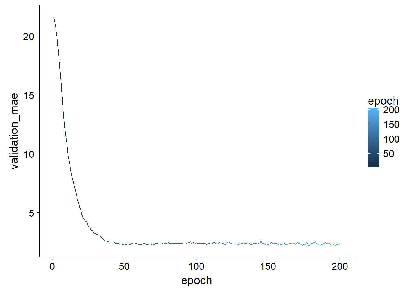
average_mae_history %>%
ggplot(aes(x = epoch, y = validation_mae, color = epoch))+
    geom_smooth()
## `geom_smooth()` using method = 'loess'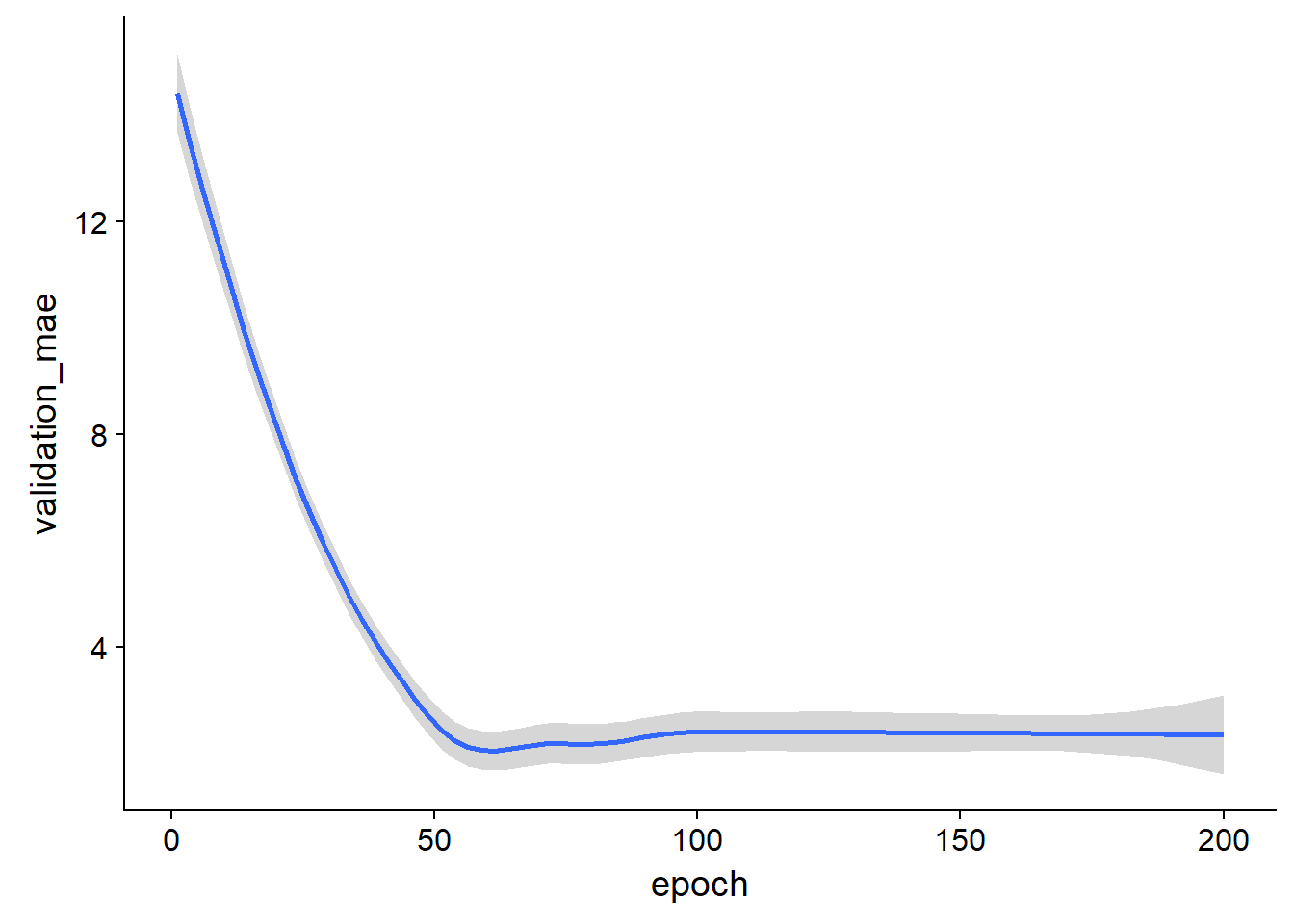
The benefit of this is that you are plotting the mean behaviour of the training at each epoch over all folds
Get results
Once we are happy with our model we can pull out all the results like this:
tidy_cross_val %>%
select(train,predictions) %>%
mutate(train = train %>% map(as_tibble)) %>%
unnest(.drop = TRUE) %>%
head()
## # A tibble: 6 x 15
## predictions V1 V2 V3 V4 V5 V6 V7 V8
## <dbl> <dbl> <dbl> <dbl> <dbl> <dbl> <dbl> <dbl> <dbl>
## 1 16.7 -0.272 -0.483 -0.435 -0.257 -0.165 -0.176 0.812 0.117
## 2 54.0 0.125 -0.483 1.03 -0.257 0.628 -1.83 1.11 -1.19
## 3 21.4 -0.401 -0.483 -0.868 -0.257 -0.361 -0.324 -1.24 1.11
## 4 18.6 -0.00563 -0.483 1.03 -0.257 1.33 0.153 0.694 -0.578
## 5 18.8 -0.375 -0.483 -0.547 -0.257 -0.549 -0.788 0.189 0.483
## 6 10.8 0.589 -0.483 1.03 -0.257 1.22 -1.03 1.11 -1.06
## # ... with 6 more variables: V9 <dbl>, V10 <dbl>, V11 <dbl>, V12 <dbl>,
## # V13 <dbl>, target <dbl>But we have only predicted on the training data in our function and we used the model trained only on that fold… Instead it would make a lot more sense to train the model on all the data now that we have tested and tuned the model (possibly censor bad folds?)
Using all the data
Run model:
train <-
    train_data %>%
    as_tibble() %>%
    bind_cols(target = train_targets)

test <-
    test_data %>%
    as_tibble() %>%
bind_cols(target = test_targets)

results <-
    define_compile_train_predict(train,test,epochs = 100)

print('mae:')
## [1] "mae:"results$mae## [1] 2.429138print('loss:')## [1] "loss:"results$loss## [1] 14.56804results$plot_outp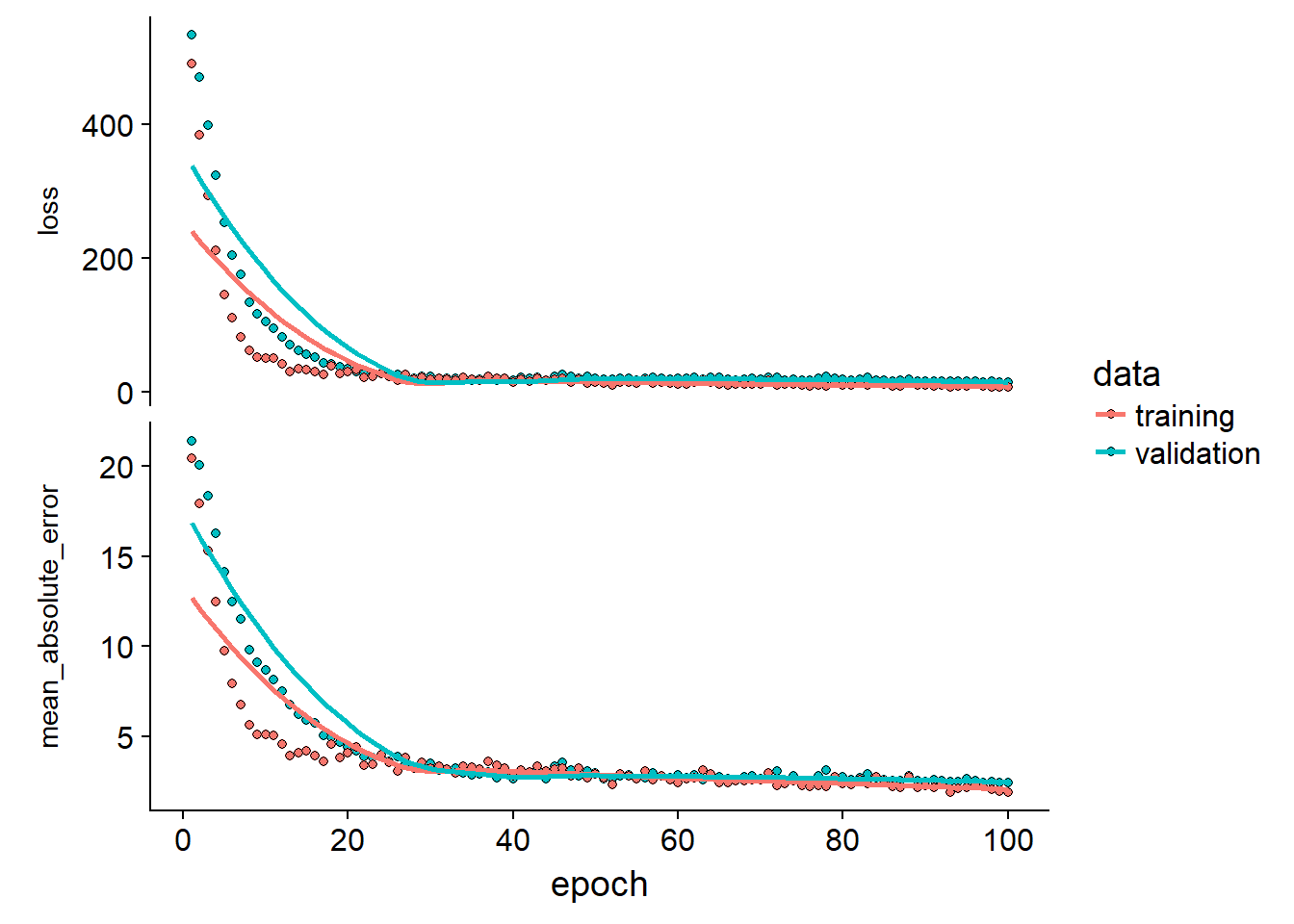
Get predictions:
output_data <-
bind_cols(predictions = results$predictions,train["target"],train)

output_data %>% head
## # A tibble: 6 x 16
## predictions target V1 V2 V3 V4 V5 V6 V7
## <dbl> <dbl> <dbl> <dbl> <dbl> <dbl> <dbl> <dbl> <dbl>
## 1 17.3 15.2 -0.272 -0.483 -0.435 -0.257 -0.165 -0.176 0.812
## 2 43.4 42.3 -0.403 2.99 -1.33 -0.257 -1.21 1.89 -1.91
## 3 51.4 50.0 0.125 -0.483 1.03 -0.257 0.628 -1.83 1.11
## 4 22.3 21.1 -0.401 -0.483 -0.868 -0.257 -0.361 -0.324 -1.24
## 5 18.4 17.7 -0.00563 -0.483 1.03 -0.257 1.33 0.153 0.694
## 6 20.8 18.5 -0.375 -0.483 -0.547 -0.257 -0.549 -0.788 0.189
## # ... with 7 more variables: V8 <dbl>, V9 <dbl>, V10 <dbl>, V11 <dbl>,
## # V12 <dbl>, V13 <dbl>, target1 <dbl>Let’s visualize the accuracy of this model:
output_data %>%
  arrange(target) %>%
  mutate(perfect = seq(5,50,length.out = nrow(.))) %>%
  mutate(estimate = ifelse(target > predictions,"underestimated","overestimated")) %>%
  select(predictions,target,estimate,perfect) %>%
  ggplot()+
  geom_point(aes(x = predictions, y = target, color = estimate))+
  geom_line(aes(x=perfect, y = perfect))+
  ggtitle("Model accuracy")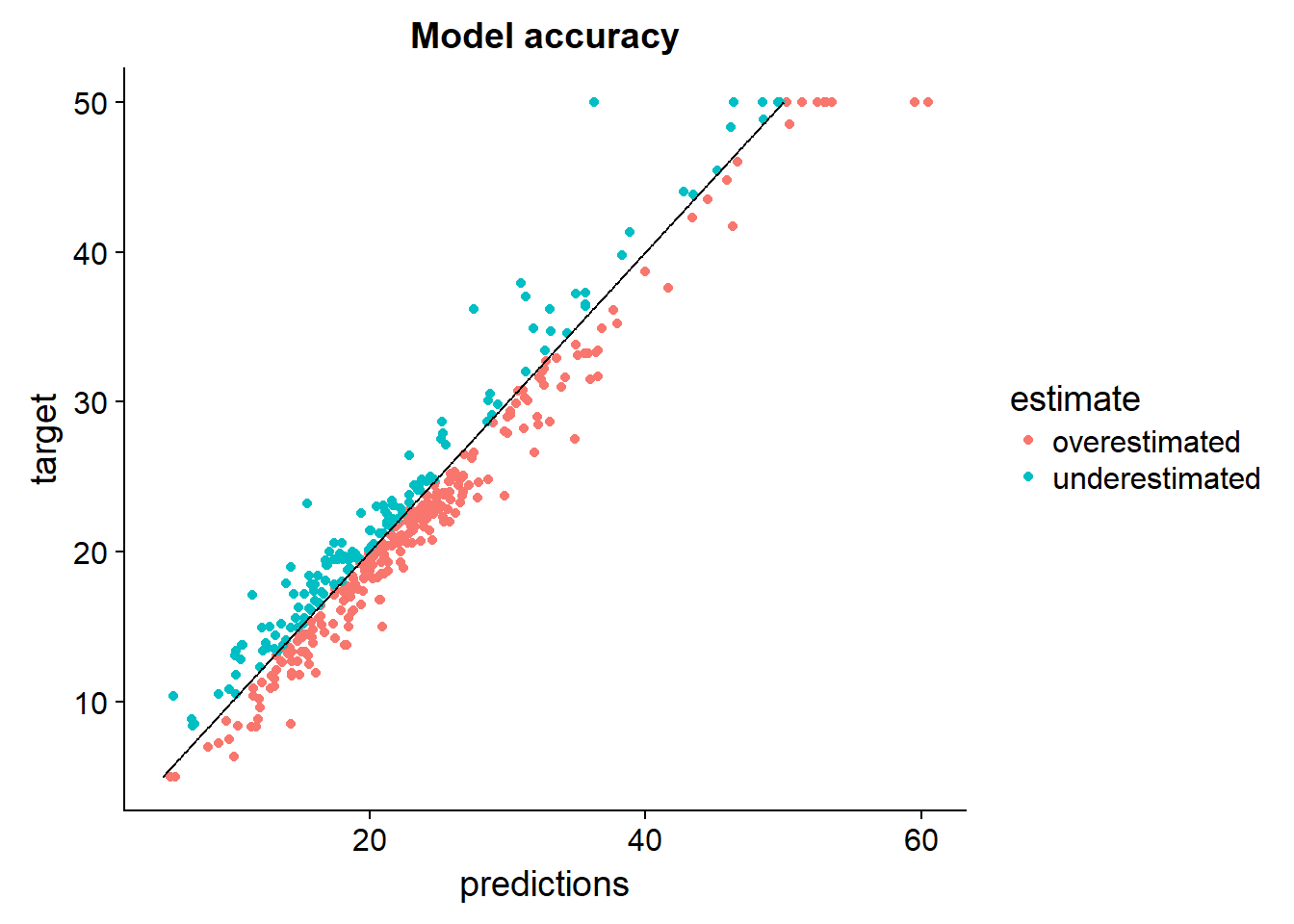
What can we say about the bias of the model:
output_data %>%
  arrange(target) %>%
  mutate(perfect = seq(5,50,length.out = nrow(.))) %>%
  mutate(estimate = ifelse(target > predictions,"underestimated","overestimated")) %>%
  select(predictions,target,estimate,perfect) %>%
  group_by(estimate) %>%
  tally %>%
  ggplot()+
  geom_bar(aes(x= estimate, y=n, fill = estimate),stat="identity")+
  ggtitle("Low model error but upward bias")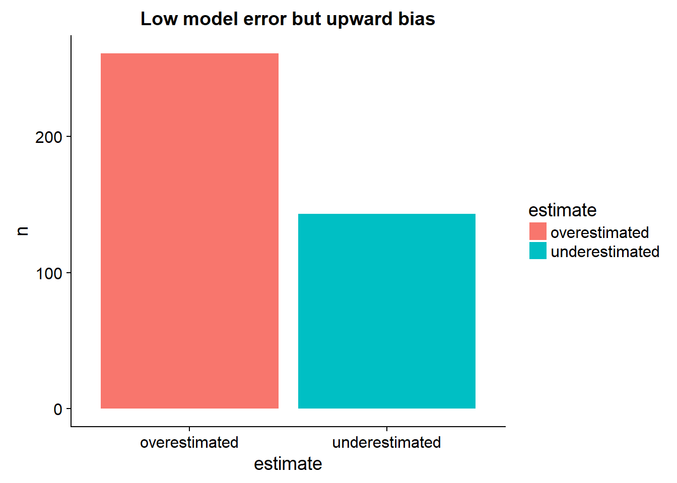
Benchmark vs Gradient boosting machines
train <-
    train_data %>%
    as_tibble() %>%
    bind_cols(target = train_targets %>% as.numeric() )

test <-
    test_data %>%
    as_tibble() %>%
bind_cols(target = test_targets %>% as.numeric() )

tr_contrl <- caret::trainControl(method = 'cv', number = 5)

results <-
caret::train(form = target~., data = train,method = 'gbm',trControl = tr_contrl)
results %>% summary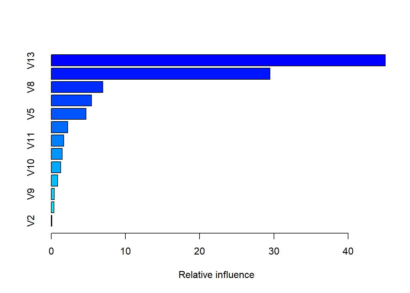
##     var     rel.inf
## V13 V13 45.00698622
## V6   V6 29.45790750
## V8   V8  6.97044377
## V1   V1  5.42153107
## V5   V5  4.70147030
## V7   V7  2.23913360
## V11 V11  1.66965671
## V12 V12  1.46723050
## V10 V10  1.28689723
## V4   V4  0.87476817
## V9   V9  0.42687149
## V3   V3  0.37745176
## V2 V2 0.09965169results## Stochastic Gradient Boosting
##
## 404 samples
## 13 predictor
##
## No pre-processing
## Resampling: Cross-Validated (5 fold)
## Summary of sample sizes: 323, 323, 323, 323, 324
## Resampling results across tuning parameters:
##
## interaction.depth n.trees RMSE Rsquared MAE
## 1 50 4.397289 0.7634246 2.947976
## 1 100 3.964773 0.8032464 2.700262
## 1 150 3.862273 0.8106288 2.670015
## 2 50 3.868630 0.8136770 2.621053
## 2 100 3.638292 0.8332715 2.537585
## 2 150 3.562024 0.8394754 2.497162
## 3 50 3.611696 0.8389383 2.463967
## 3 100 3.350380 0.8589171 2.345241
## 3 150 3.214416 0.8688836 2.286692
##
## Tuning parameter 'shrinkage' was held constant at a value of 0.1
##
## Tuning parameter 'n.minobsinnode' was held constant at a value of 10
## RMSE was used to select the optimal model using the smallest value.
## The final values used for the model were n.trees = 150,
## interaction.depth = 3, shrinkage = 0.1 and n.minobsinnode = 10.So the gradient boosted machine using k-fold can get around 2.4-2.9 MAE and the GBM model is historically the best tabular learning paradigm in the average kaggle contest the last couple of years (around 2016). Our model learned the same ammount of accuracy also using cross-validation.

Let’s visualize the accuracy of this model:
output_data <-
  train %>%
  as_tibble() %>%
  mutate(predictions = results %>% predict(newData=train %>% select(-target))) %>%
  select(target,predictions)

output_data %>%
  arrange(target) %>%
  mutate(perfect = seq(5,50,length.out = nrow(.))) %>%
  mutate(estimate = ifelse(target > predictions,"underestimated","overestimated")) %>%
  select(predictions,target,estimate,perfect) %>%
  ggplot()+
  geom_point(aes(x = predictions, y = target, color = estimate))+
  geom_line(aes(x=perfect, y = perfect))+
  ggtitle("Model accuracy GBM")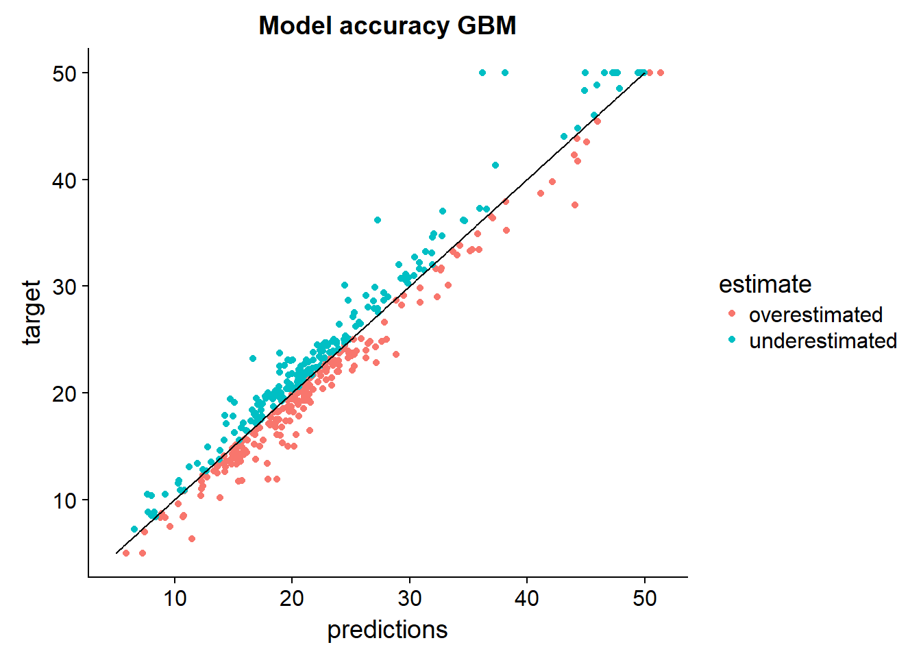
What can we say about the bias of the model:
output_data %>%
  arrange(target) %>%
  mutate(perfect = seq(5,50,length.out = nrow(.))) %>%
  mutate(estimate = ifelse(target > predictions,"underestimated","overestimated")) %>%
  select(predictions,target,estimate,perfect) %>%
  group_by(estimate) %>%
  tally %>%
  ggplot()+
  geom_bar(aes(x= estimate, y=n, fill = estimate),stat="identity")+
  ggtitle("GBM has low model error and less bias")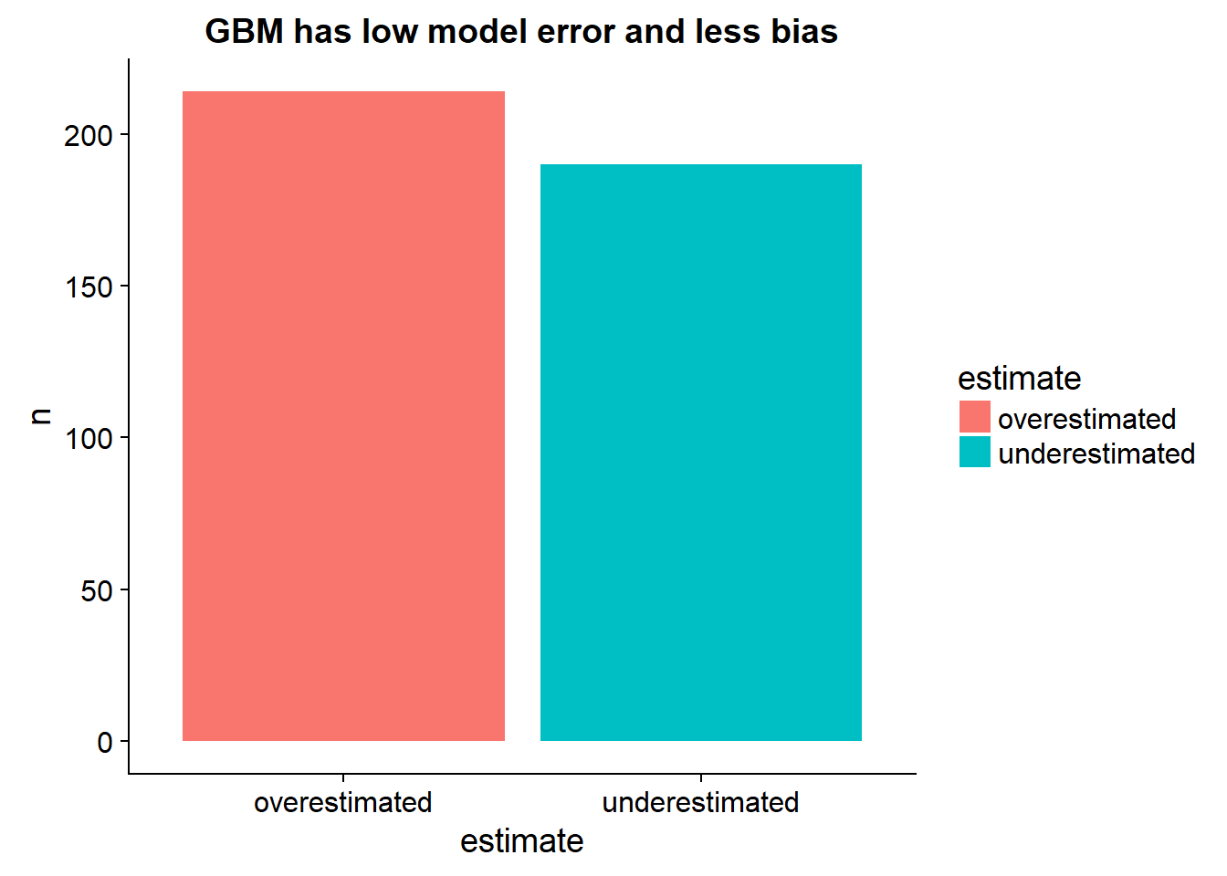
Time series models using LSTM together with an inference network
Besides a dense feedforward network we can also predict time series movements of house prices using a LSTM network. This will allow us to predict the average move in house prices over the next couple of months
Read in the data
All residential home sales in Ames, Iowa between 2006 and 2010
# https://www.openintro.org/stat/data/ames.csv

if(!file.exists("../../static/data/cencus_data.csv")){
    download.file(url = 'https://www.openintro.org/stat/data/ames.csv',destfile = '../../static/data/cencus_data.csv')
}
So we can tell that in this data we have primarily just a time index and a value. This is enough for us but we need to pre-process and label these 2 fields in a tidy dataframe before we start ironing out the model process.
Read in the data
housing_time_series <-
    data.table::fread(input = "../../static/data/cencus_data.csv")

housing_time_series %>% head
## Order PID MS.SubClass MS.Zoning Lot.Frontage Lot.Area Street
## 1: 1 526301100 20 RL 141 31770 Pave
## 2: 2 526350040 20 RH 80 11622 Pave
## 3: 3 526351010 20 RL 81 14267 Pave
## 4: 4 526353030 20 RL 93 11160 Pave
## 5: 5 527105010 60 RL 74 13830 Pave
## 6: 6 527105030 60 RL 78 9978 Pave
## Alley Lot.Shape Land.Contour Utilities Lot.Config Land.Slope
## 1: NA IR1 Lvl AllPub Corner Gtl
## 2: NA Reg Lvl AllPub Inside Gtl
## 3: NA IR1 Lvl AllPub Corner Gtl
## 4: NA Reg Lvl AllPub Corner Gtl
## 5: NA IR1 Lvl AllPub Inside Gtl
## 6: NA IR1 Lvl AllPub Inside Gtl
## Neighborhood Condition.1 Condition.2 Bldg.Type House.Style Overall.Qual
## 1: NAmes Norm Norm 1Fam 1Story 6
## 2: NAmes Feedr Norm 1Fam 1Story 5
## 3: NAmes Norm Norm 1Fam 1Story 6
## 4: NAmes Norm Norm 1Fam 1Story 7
## 5: Gilbert Norm Norm 1Fam 2Story 5
## 6: Gilbert Norm Norm 1Fam 2Story 6
## Overall.Cond Year.Built Year.Remod.Add Roof.Style Roof.Matl
## 1: 5 1960 1960 Hip CompShg
## 2: 6 1961 1961 Gable CompShg
## 3: 6 1958 1958 Hip CompShg
## 4: 5 1968 1968 Hip CompShg
## 5: 5 1997 1998 Gable CompShg
## 6: 6 1998 1998 Gable CompShg
## Exterior.1st Exterior.2nd Mas.Vnr.Type Mas.Vnr.Area Exter.Qual
## 1: BrkFace Plywood Stone 112 TA
## 2: VinylSd VinylSd None 0 TA
## 3: Wd Sdng Wd Sdng BrkFace 108 TA
## 4: BrkFace BrkFace None 0 Gd
## 5: VinylSd VinylSd None 0 TA
## 6: VinylSd VinylSd BrkFace 20 TA
## Exter.Cond Foundation Bsmt.Qual Bsmt.Cond Bsmt.Exposure BsmtFin.Type.1
## 1: TA CBlock TA Gd Gd BLQ
## 2: TA CBlock TA TA No Rec
## 3: TA CBlock TA TA No ALQ
## 4: TA CBlock TA TA No ALQ
## 5: TA PConc Gd TA No GLQ
## 6: TA PConc TA TA No GLQ
## BsmtFin.SF.1 BsmtFin.Type.2 BsmtFin.SF.2 Bsmt.Unf.SF Total.Bsmt.SF
## 1: 639 Unf 0 441 1080
## 2: 468 LwQ 144 270 882
## 3: 923 Unf 0 406 1329
## 4: 1065 Unf 0 1045 2110
## 5: 791 Unf 0 137 928
## 6: 602 Unf 0 324 926
## Heating Heating.QC Central.Air Electrical X1st.Flr.SF X2nd.Flr.SF
## 1: GasA Fa Y SBrkr 1656 0
## 2: GasA TA Y SBrkr 896 0
## 3: GasA TA Y SBrkr 1329 0
## 4: GasA Ex Y SBrkr 2110 0
## 5: GasA Gd Y SBrkr 928 701
## 6: GasA Ex Y SBrkr 926 678
## Low.Qual.Fin.SF Gr.Liv.Area Bsmt.Full.Bath Bsmt.Half.Bath Full.Bath
## 1: 0 1656 1 0 1
## 2: 0 896 0 0 1
## 3: 0 1329 0 0 1
## 4: 0 2110 1 0 2
## 5: 0 1629 0 0 2
## 6: 0 1604 0 0 2
## Half.Bath Bedroom.AbvGr Kitchen.AbvGr Kitchen.Qual TotRms.AbvGrd
## 1: 0 3 1 TA 7
## 2: 0 2 1 TA 5
## 3: 1 3 1 Gd 6
## 4: 1 3 1 Ex 8
## 5: 1 3 1 TA 6
## 6: 1 3 1 Gd 7
## Functional Fireplaces Fireplace.Qu Garage.Type Garage.Yr.Blt
## 1: Typ 2 Gd Attchd 1960
## 2: Typ 0 NA Attchd 1961
## 3: Typ 0 NA Attchd 1958
## 4: Typ 2 TA Attchd 1968
## 5: Typ 1 TA Attchd 1997
## 6: Typ 1 Gd Attchd 1998
## Garage.Finish Garage.Cars Garage.Area Garage.Qual Garage.Cond
## 1: Fin 2 528 TA TA
## 2: Unf 1 730 TA TA
## 3: Unf 1 312 TA TA
## 4: Fin 2 522 TA TA
## 5: Fin 2 482 TA TA
## 6: Fin 2 470 TA TA
## Paved.Drive Wood.Deck.SF Open.Porch.SF Enclosed.Porch X3Ssn.Porch
## 1: P 210 62 0 0
## 2: Y 140 0 0 0
## 3: Y 393 36 0 0
## 4: Y 0 0 0 0
## 5: Y 212 34 0 0
## 6: Y 360 36 0 0
## Screen.Porch Pool.Area Pool.QC Fence Misc.Feature Misc.Val Mo.Sold
## 1: 0 0 NA NA NA 0 5
## 2: 120 0 NA MnPrv NA 0 6
## 3: 0 0 NA NA Gar2 12500 6
## 4: 0 0 NA NA NA 0 4
## 5: 0 0 NA MnPrv NA 0 3
## 6: 0 0 NA NA NA 0 6
## Yr.Sold Sale.Type Sale.Condition SalePrice
## 1: 2010 WD Normal 215000
## 2: 2010 WD Normal 105000
## 3: 2010 WD Normal 172000
## 4: 2010 WD Normal 244000
## 5: 2010 WD Normal 189900
## 6: 2010 WD Normal 195500Process data
We need to:
- Deal with NA’s
- Create vectorized tensors
- Scale tensors into small values
- Make sure all tensors have homogeneous scale
- Split data into time series and inference sets
We need to create a date formatted feature and we need to parse our categorical features to vectorized tensors. The reason we do this is because we want to fit 2 different models at the same time. One model will predict the price of a property based on the autocorrelations in the data, much like an arima or ets model would (we can use LSTM networks for this), and the other model will predict the price of the home given the 1D tensor data describing the property - street, size, zoning etc.
Let’s count NA’s
NA_info <-
housing_time_series %>%
  as_tibble() %>%
map_df(~.x %>% is.na %>% sum) %>%
gather(key = "feature", value = "count_NA") %>%
arrange(-count_NA)
So out of the 82 columns in the data the colums that have more than 50 NA’s are
remove_features_str <-
NA_info %>%
filter(count_NA>50) %>%
pull(feature)

remove_features_str
## [1] "Pool.QC" "Misc.Feature" "Alley" "Fence"
## [5] "Fireplace.Qu" "Lot.Frontage" "Garage.Yr.Blt" "Garage.Qual"
## [9] "Garage.Cond" "Garage.Type" "Garage.Finish" "Bsmt.Qual"
## [13] "Bsmt.Cond" "Bsmt.Exposure" "BsmtFin.Type.1" "BsmtFin.Type.2"remove_features_str %>% length()## [1] 16For the sake of this tutorial we will just throw these away but it may be useful to impute these using nearest neighbors or mean imputations. You can leverage something like the mice package.
Remove the columns and remove leftover NA observations
housing_time_series_cleaned <-
housing_time_series %>%
select(-which(names(.) %in% remove_features_str)) %>%
na.omit() %>%
select(SalePrice,Yr.Sold,Mo.Sold,everything()) %>%
select(-PID,-Order
# ,-Year.Built,-Year.Remod.Add
)

housing_time_series_cleaned %>% dim()
## [1] 2904 64So what we are left with is a table with 66 features and 2904 samples…
Split the data for 2 models
We want to train a model to predict house prices using the descriptive features and also train an lstm model to predict future price movements.
First we need to split test train sets:
split_data <-
caret::createDataPartition(housing_time_series_cleaned$SalePrice, p = 0.8, list = FALSE)

train <-
housing_time_series_cleaned[split_data,]

test <-
housing_time_series_cleaned[-split_data,]
It’s important that our time series does not have missing months since we will lag time vectors later on… If there were missing months the auto correlation of say n month lags will get mixed up with n+1 month lags. Let’s check this:
interaction(test$Yr.Sold,test$Mo.Sold) %>% unique()## [1] 2010.5 2010.2 2010.1 2010.6 2010.4 2010.3 2010.7 2009.10
## [9] 2009.6 2009.5 2009.12 2009.7 2009.8 2009.3 2009.2 2009.9
## [17] 2009.11 2009.4 2009.1 2008.5 2008.8 2008.10 2008.7 2008.6
## [25] 2008.3 2008.11 2008.9 2008.2 2008.1 2008.4 2008.12 2007.5
## [33] 2007.8 2007.3 2007.7 2007.6 2007.10 2007.1 2007.9 2007.4
## [41] 2007.11 2007.12 2007.2 2006.8 2006.12 2006.9 2006.7 2006.1
## [49] 2006.3 2006.2 2006.6 2006.4 2006.11 2006.5 2006.10
## 60 Levels: 2006.1 2007.1 2008.1 2009.1 2010.1 2006.2 2007.2 ... 2010.12interaction(train$Yr.Sold,train$Mo.Sold) %>% unique()## [1] 2010.5 2010.6 2010.4 2010.3 2010.1 2010.2 2010.7 2009.7
## [9] 2009.8 2009.6 2009.10 2009.11 2009.9 2009.2 2009.12 2009.5
## [17] 2009.4 2009.3 2009.1 2008.5 2008.6 2008.4 2008.10 2008.7
## [25] 2008.11 2008.8 2008.9 2008.3 2008.12 2008.1 2008.2 2007.3
## [33] 2007.4 2007.2 2007.10 2007.7 2007.8 2007.6 2007.5 2007.9
## [41] 2007.11 2007.1 2007.12 2006.5 2006.6 2006.10 2006.3 2006.11
## [49] 2006.2 2006.7 2006.1 2006.9 2006.8 2006.12 2006.4
## 60 Levels: 2006.1 2007.1 2008.1 2009.1 2010.1 2006.2 2007.2 ... 2010.12Since both sets have all 60 months we don’t have any problems here…
For the LSTM model we need only the time index and the value:
For the time series model we are going to train on the moving average monthly house price so the complete model can use this in predictions
LSTM_train <-
train %>%
select(SalePrice,Yr.Sold,Mo.Sold) %>%
tidyr::unite(col = index,Yr.Sold,Mo.Sold,sep="-") %>%
mutate(index = index %>% zoo::as.yearmon() %>% as_date()) %>%
rename(value = SalePrice) %>%
group_by(index) %>%
summarise(value = mean(value,na.rm = TRUE)) %>%
as_tbl_time(index = index)

LSTM_test <-
test %>%
select(SalePrice,Yr.Sold,Mo.Sold) %>%
tidyr::unite(col = index,Yr.Sold,Mo.Sold,sep="-") %>%
mutate(index = index %>% zoo::as.yearmon() %>% as_date()) %>%
rename(value = SalePrice) %>%
group_by(index) %>%
summarise(value = mean(value,na.rm = TRUE)) %>%
as_tbl_time(index = index)

LSTM_train %>% head
## # A time tibble: 6 x 2
## # Index: index
## index value
## <date> <dbl>
## 1 2006-01-01 212711.
## 2 2006-02-01 182493.
## 3 2006-03-01 180162.
## 4 2006-04-01 170443.
## 5 2006-05-01 170079.
## 6 2006-06-01 178162.Function that one_hot encodes classes for prediction
one_hot_categorical_inputs_fn <- function(tibble_df) {

one_hot_list <-
tibble_df %>%
map_if(is.character,as_factor) %>%
map_if(is.factor,keras::to_categorical)

bind_binary_classes <-
one_hot_list %>%
purrr::keep(is.matrix) %>%
reduce(cbind)

bind_numeric_features <-
one_hot_list %>%
purrr::discard(is.matrix) %>%
reduce(cbind) %>%
as.matrix()

return(cbind(bind_numeric_features,bind_binary_classes))

}
Before we cast everything to numeric we should scale these numeric variables since the new sparse matrices will have 1’s and 0’s:
Function that will scale all the numeric variables
scale_numerics_fn <- function(df_in, mean = NULL, std = NULL,...) {

numeric_cols <-
df_in %>% map_lgl(is.numeric)

scaled_numeric <-
df_in %>%
select_if(numeric_cols)

if(is.null(mean) | is.null(std)) {
mean <- apply(scaled_numeric, 2, mean)
std <- apply(scaled_numeric, 2, sd)
}

recombined <-
cbind(
scale(scaled_numeric, center = mean, scale = std),
df_in %>% select_if(!numeric_cols)
)

return(list(recombined = recombined,mean = mean, std = std))

}
Scale numerics… (Remember that the test set must be scaled using the training scales otherwise you wouldn’t be predicting using the same data scale as trained)
Here we will start out with the original cleaned data again because we want to spread the same number of classes in the train and test sets
data_scaled <-
    housing_time_series_cleaned %>%
    select(-Yr.Sold,-Mo.Sold,-SalePrice)

data_scaled_outp <-
data_scaled %>%
scale_numerics_fn

data_scaled <-
    data_scaled_outp$recombined

inference_X <-
data_scaled %>%
one_hot_categorical_inputs_fn()

inference_target <-
housing_time_series_cleaned %>%
select(SalePrice) %>%
as.matrix()

inference_X %>% head
## out
## [1,] -0.87715441 2.74965990 -0.06154026 -0.5089121 -0.3685560 -1.1560238
## [2,] -0.87715441 0.18952801 -0.77071847 0.3889498 -0.3354663 -1.1080859
## [3,] -0.87715441 0.52561839 -0.06154026 0.3889498 -0.4347354 -1.2518997
## [4,] -0.87715441 0.13082338 0.64763795 -0.5089121 -0.1038383 -0.7725204
## [5,] 0.05903575 0.47009041 -0.77071847 -0.5089121 0.8557633 0.6656175
## [6,] 0.05903575 -0.01936899 -0.06154026 0.3889498 0.8888530 0.6656175
##
## [1,] 0.05579978 0.43144278 -0.2947952 -0.2670621 0.06612207 1.2816766
## [2,] -0.56928686 0.05583144 0.5533971 -0.6565320 -0.38356992 -0.6750520
## [3,] 0.03347525 1.05526512 -0.2947952 -0.3467782 0.63164381 0.4397683
## [4,] -0.56928686 1.36717629 -0.2947952 1.1086092 2.40542888 2.4505644
## [5,] -0.56928686 0.76531953 -0.2947952 -0.9594530 -0.27909603 -0.5926635
## [6,] -0.45766424 0.35017015 -0.2947952 -0.5335415 -0.28363837 -0.5978128
##
## [1,] -0.7820247 -0.1014432 0.3137316 1.0827555 -0.2503599 -1.019769
## [2,] -0.7820247 -0.1014432 -1.1925373 -0.8217399 -0.2503599 -1.019769
## [3,] -0.7820247 -0.1014432 -0.3343604 -0.8217399 -0.2503599 -1.019769
## [4,] -0.7820247 -0.1014432 1.2135291 1.0827555 -0.2503599 0.793709
## [5,] 0.8554028 -0.1014432 0.2602194 -0.8217399 -0.2503599 0.793709
## [6,] 0.8016783 -0.1014432 0.2106711 -0.8217399 -0.2503599 0.793709
##
## [1,] -0.7518758 0.1759575 -0.2073247 0.3546094 2.1638512 0.3093533
## [2,] -0.7518758 -1.0320345 -0.2073247 -0.9167310 -0.9240229 -1.0040415
## [3,] 1.2421400 0.1759575 -0.2073247 -0.2810608 -0.9240229 -1.0040415
## [4,] 1.2421400 0.1759575 -0.2073247 0.9902796 2.1638512 0.3093533
## [5,] 1.2421400 0.1759575 -0.2073247 -0.2810608 0.6199141 0.3093533
## [6,] 1.2421400 0.1759575 -0.2073247 0.3546094 0.6199141 0.3093533
##
## [1,] 0.2588252 0.9160874 0.2215652 -0.3587571 -0.1035821 -0.2866842
## [2,] 1.1972919 0.3632432 -0.7032610 -0.3587571 -0.1035821 1.8440946
## [3,] -0.7446839 2.3613800 -0.1662651 -0.3587571 -0.1035821 -0.2866842
## [4,] 0.2309499 -0.7424451 -0.7032610 -0.3587571 -0.1035821 -0.2866842
## [5,] 0.0451149 0.9318829 -0.1960982 -0.3587571 -0.1035821 -0.2866842
## [6,] -0.0106356 2.1007535 -0.1662651 -0.3587571 -0.1035821 -0.2866842
##
## [1,] -0.06330281 -0.08980944 0 1 0 0 0 0 0 0 0 1 0 0 1 0 0 0 0 1 0 0 0 0 1
## [2,] -0.06330281 -0.08980944 0 0 1 0 0 0 0 0 0 1 0 0 0 1 0 0 0 1 0 0 0 0 1
## [3,] -0.06330281 21.88417774 0 1 0 0 0 0 0 0 0 1 0 0 1 0 0 0 0 1 0 0 0 0 1
## [4,] -0.06330281 -0.08980944 0 1 0 0 0 0 0 0 0 1 0 0 0 1 0 0 0 1 0 0 0 0 1
## [5,] -0.06330281 -0.08980944 0 1 0 0 0 0 0 0 0 1 0 0 1 0 0 0 0 1 0 0 0 0 1
## [6,] -0.06330281 -0.08980944 0 1 0 0 0 0 0 0 0 1 0 0 1 0 0 0 0 1 0 0 0 0 1
##
## [1,] 0 0 0 1 0 0 0 0 0 1 0 0 0 1 0 0 0 0 0 0 0 0 0 0 0 0 0 0 0 0 0 0 0 0 0
## [2,] 0 0 0 0 1 0 0 0 0 1 0 0 0 1 0 0 0 0 0 0 0 0 0 0 0 0 0 0 0 0 0 0 0 0 0
## [3,] 0 0 0 1 0 0 0 0 0 1 0 0 0 1 0 0 0 0 0 0 0 0 0 0 0 0 0 0 0 0 0 0 0 0 0
## [4,] 0 0 0 1 0 0 0 0 0 1 0 0 0 1 0 0 0 0 0 0 0 0 0 0 0 0 0 0 0 0 0 0 0 0 0
## [5,] 0 0 0 0 1 0 0 0 0 1 0 0 0 0 1 0 0 0 0 0 0 0 0 0 0 0 0 0 0 0 0 0 0 0 0
## [6,] 0 0 0 0 1 0 0 0 0 1 0 0 0 0 1 0 0 0 0 0 0 0 0 0 0 0 0 0 0 0 0 0 0 0 0
##
## [1,] 0 0 0 0 0 0 0 1 0 0 0 0 0 0 0 0 0 1 0 0 0 0 0 0 0 0 1 0 0 0 0 0 1 0 0
## [2,] 0 0 0 0 0 0 0 0 1 0 0 0 0 0 0 0 0 1 0 0 0 0 0 0 0 0 1 0 0 0 0 0 1 0 0
## [3,] 0 0 0 0 0 0 0 1 0 0 0 0 0 0 0 0 0 1 0 0 0 0 0 0 0 0 1 0 0 0 0 0 1 0 0
## [4,] 0 0 0 0 0 0 0 1 0 0 0 0 0 0 0 0 0 1 0 0 0 0 0 0 0 0 1 0 0 0 0 0 1 0 0
## [5,] 0 0 0 0 0 0 0 1 0 0 0 0 0 0 0 0 0 1 0 0 0 0 0 0 0 0 1 0 0 0 0 0 0 1 0
## [6,] 0 0 0 0 0 0 0 1 0 0 0 0 0 0 0 0 0 1 0 0 0 0 0 0 0 0 1 0 0 0 0 0 0 1 0
##
## [1,] 0 0 0 0 0 0 1 0 0 0 0 0 0 1 0 0 0 0 0 0 0 0 1 0 0 0 0 0 0 0 0 0 0 0 0
## [2,] 0 0 0 0 0 0 0 1 0 0 0 0 0 1 0 0 0 0 0 0 0 0 0 1 0 0 0 0 0 0 0 0 0 0 0
## [3,] 0 0 0 0 0 0 1 0 0 0 0 0 0 1 0 0 0 0 0 0 0 0 0 0 1 0 0 0 0 0 0 0 0 0 0
## [4,] 0 0 0 0 0 0 1 0 0 0 0 0 0 1 0 0 0 0 0 0 0 0 1 0 0 0 0 0 0 0 0 0 0 0 0
## [5,] 0 0 0 0 0 0 0 1 0 0 0 0 0 1 0 0 0 0 0 0 0 0 0 1 0 0 0 0 0 0 0 0 0 0 0
## [6,] 0 0 0 0 0 0 0 1 0 0 0 0 0 1 0 0 0 0 0 0 0 0 0 1 0 0 0 0 0 0 0 0 0 0 0
##
## [1,] 0 0 0 0 1 0 0 0 0 0 0 0 0 0 0 0 0 0 0 0 0 0 1 0 0 0 0 0 1 0 0 0 0 1 0
## [2,] 0 0 0 0 0 1 0 0 0 0 0 0 0 0 0 0 0 0 0 0 0 0 0 1 0 0 0 0 1 0 0 0 0 1 0
## [3,] 0 0 0 0 0 0 1 0 0 0 0 0 0 0 0 0 0 0 0 0 0 0 0 0 1 0 0 0 1 0 0 0 0 1 0
## [4,] 0 0 0 0 0 0 0 1 0 0 0 0 0 0 0 0 0 0 0 0 0 0 0 1 0 0 0 0 0 1 0 0 0 1 0
## [5,] 0 0 0 0 0 1 0 0 0 0 0 0 0 0 0 0 0 0 0 0 0 0 0 1 0 0 0 0 1 0 0 0 0 1 0
## [6,] 0 0 0 0 0 1 0 0 0 0 0 0 0 0 0 0 0 0 0 0 0 0 0 0 1 0 0 0 1 0 0 0 0 1 0
##
## [1,] 0 0 0 0 1 0 0 0 0 0 0 1 0 0 0 0 0 0 1 0 0 0 0 0 1 0 0 1 0 0 0 0 0 0 1
## [2,] 0 0 0 0 1 0 0 0 0 0 0 1 0 0 0 0 0 0 0 1 0 0 0 0 1 0 0 1 0 0 0 0 0 0 1
## [3,] 0 0 0 0 1 0 0 0 0 0 0 1 0 0 0 0 0 0 0 1 0 0 0 0 1 0 0 1 0 0 0 0 0 0 0
## [4,] 0 0 0 0 1 0 0 0 0 0 0 1 0 0 0 0 0 0 0 0 1 0 0 0 1 0 0 1 0 0 0 0 0 0 0
## [5,] 0 0 0 0 0 1 0 0 0 0 0 1 0 0 0 0 0 0 0 0 0 1 0 0 1 0 0 1 0 0 0 0 0 0 1
## [6,] 0 0 0 0 0 1 0 0 0 0 0 1 0 0 0 0 0 0 0 0 1 0 0 0 1 0 0 1 0 0 0 0 0 0 0
##
## [1,] 0 0 0 0 0 1 0 0 0 0 0 0 0 0 1 0 0 0 1 0 0 0 0 0 0 0 0 0 0 1 0 0 0 0 0
## [2,] 0 0 0 0 0 1 0 0 0 0 0 0 0 0 0 1 0 0 1 0 0 0 0 0 0 0 0 0 0 1 0 0 0 0 0
## [3,] 1 0 0 0 0 1 0 0 0 0 0 0 0 0 0 1 0 0 1 0 0 0 0 0 0 0 0 0 0 1 0 0 0 0 0
## [4,] 0 1 0 0 0 1 0 0 0 0 0 0 0 0 0 1 0 0 1 0 0 0 0 0 0 0 0 0 0 1 0 0 0 0 0
## [5,] 0 0 0 0 0 1 0 0 0 0 0 0 0 0 0 1 0 0 1 0 0 0 0 0 0 0 0 0 0 1 0 0 0 0 0
## [6,] 1 0 0 0 0 1 0 0 0 0 0 0 0 0 0 1 0 0 1 0 0 0 0 0 0 0 0 0 0 1 0 0 0 0 0inference_target %>% head## SalePrice
## [1,] 215000
## [2,] 105000
## [3,] 172000
## [4,] 244000
## [5,] 189900
## [6,] 195500inference_train_X <-
inference_X[split_data,]
inference_test_X <-
inference_X[-split_data,]
inference_train_target <-
inference_target[split_data,]
inference_test_target <-
inference_target[-split_data,]So we have 265 dimesnions on the tensor axis
So at this point we have nicely scaled and homogeneous inputs in a nice vectorized format for our tensors to learn with. The only data we have not vectorized is the time series data we will use in the LSTM model

Design inference model
Now that our data is processed we can try to build the skeleton of our inference model that we will train together with the LSTM model
We can use the same structure we used in the naive model:
define_compile_train_predict <- function(train_X,test_X,train_y,test_y,epochs = 100,shuffle = TRUE,...){

#define
base_model <-
keras_model_sequential() %>%
layer_dense(units = 128, activation = 'relu', input_shape = dim(train_X)[2]) %>% # 1 axis and nr features = number columns
layer_batch_normalization() %>%
# layer_dropout(rate = 0.2) %>%
layer_dense(units = 64, activation ='relu') %>%
layer_dense(units = 32, activation ='relu') %>%
# layer_dense(units = 25, activation ='relu') %>%
layer_dense(units = 1)

#compile
base_model %>% compile(
  loss='mse',
  optimizer='rmsprop',
    # optimizer='adam',
  metrics = c('mae')
)

#train
history <- base_model %>%
  keras::fit(train_X,
             train_y,
             epochs=epochs,
             shuffle=shuffle,
             validation_data= list(test_X, test_y),
                verbose = 0
             )

#predict
predictions <-
    base_model %>%
    keras::predict_on_batch(x = train_X)

results <-
base_model %>%
keras::evaluate(test_X, test_y, verbose = 0)

plot_outp <-
    history %>% plot

return(list(predictions = predictions, loss = results$loss, mae = results$mean_absolute_error, plot_outp = plot_outp,base_model=base_model,history = history))

}
Let’s see out of box performance of our inference network:
model_outp <-
define_compile_train_predict(train_X = inference_train_X, train_y = inference_train_target,test_X = inference_test_X, test_y = inference_test_target)

model_outp$plot_outp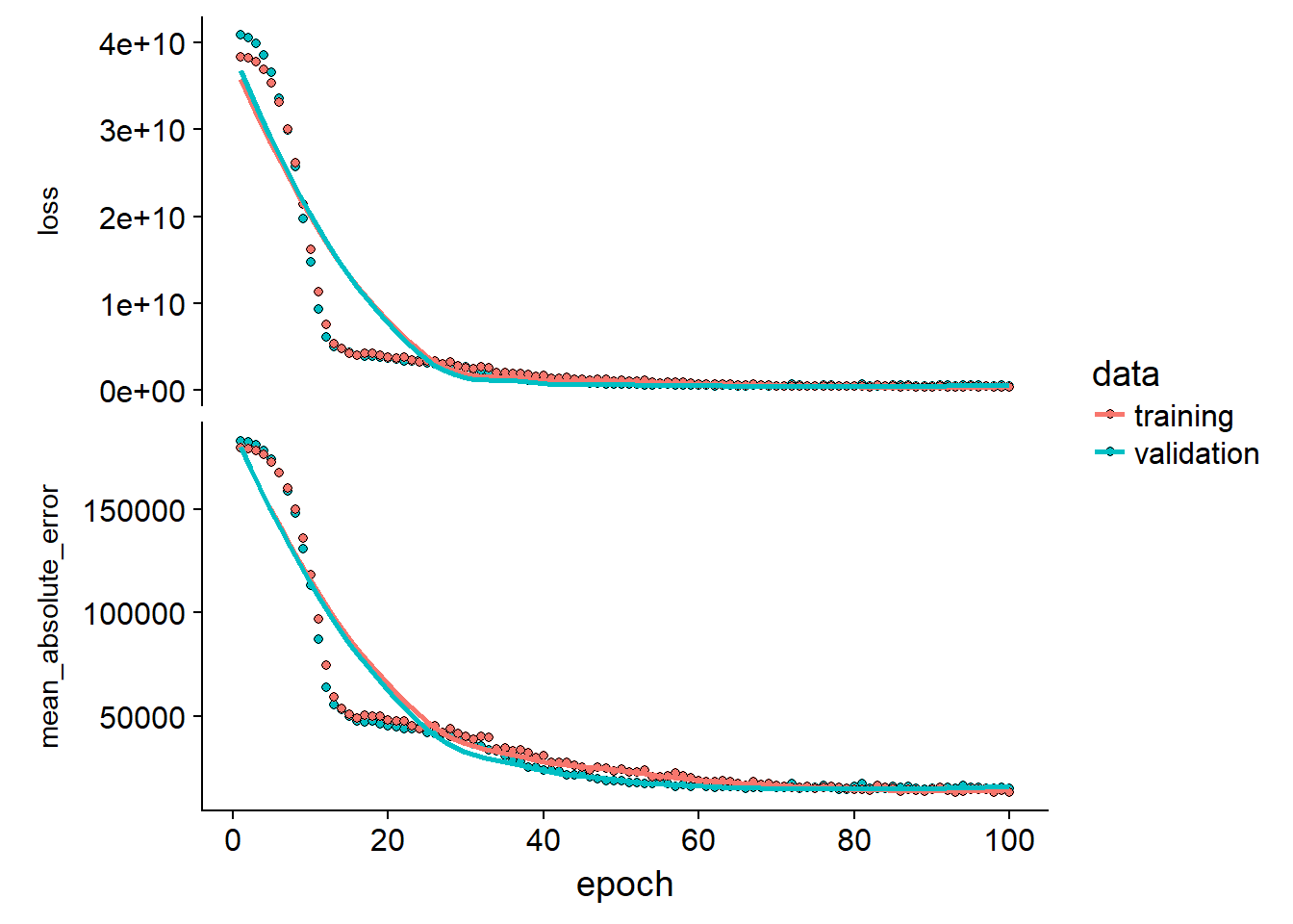
model_outp$history$metrics$val_mean_absolute_error %>% last()## [1] 14664.32This looks promising… If we calculate the MAE / average price: 8.1628129 %
This is the expected % error before we optimize the model and combine the LSTM network. I have not yet tested and tuned the network here so with some revision to the network we could potentially improve this by a lot.
Design LSTM model
Let’s start by visualizing the time series data…
Now remember we made the training time tibble:
LSTM_train %>% head## # A time tibble: 6 x 2
## # Index: index
## index value
## <date> <dbl>
## 1 2006-01-01 212711.
## 2 2006-02-01 182493.
## 3 2006-03-01 180162.
## 4 2006-04-01 170443.
## 5 2006-05-01 170079.
## 6 2006-06-01 178162.Let’s visualize the average price
LSTM_train %>%
    # filter_time("2008" ~ "end") %>%
    ggplot(aes(index, value)) +
    geom_line(color = palette_light()[[1]], alpha = 0.5) +
    geom_point(color = palette_light()[[1]]) +
    geom_smooth(method = "loess", span = 0.2, se = FALSE) +
    theme_tq()+
labs(title = 'All residential home sales in Ames, Iowa between 2006 and 2010')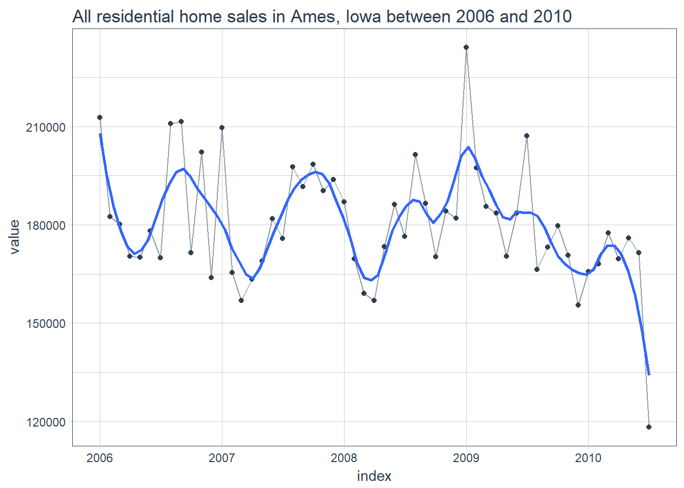
So this timeseries actually looks surprisingly stationary with expected volatility around the 2009 market crash. We will have to see if a LSTM network can make some sense out of this.
We define the handy tidy_acf function
tidy_acf <- function(data, value, lags = 0:20) {

    value_expr <- enquo(value)

    acf_values <- data %>%
        pull(value) %>%
        acf(lag.max = tail(lags, 1), plot = FALSE) %>%
        .$acf %>%
        .[,,1]

    ret <- tibble(acf = acf_values) %>%
        rowid_to_column(var = "lag") %>%
        mutate(lag = lag - 1) %>%
        filter(lag %in% lags)

    return(ret)
}

tidy_pacf <- function(data, value, lags = 0:20) {

    value_expr <- enquo(value)

    pacf_values <- data %>%
        pull(value) %>%
        pacf(lag.max = tail(lags, 1), plot = FALSE) %>%
        .$acf %>%
        .[,,1]

    ret <- tibble(pacf = pacf_values) %>%
        rowid_to_column(var = "lag") %>%
        mutate(lag = lag - 1) %>%
        filter(lag %in% lags)

    return(ret)
}
Let’s view the significant lags in the ACF and PACF
max_lag <- 100 # these are months, since our samples are sales in a month

LSTM_train %>%
    tidy_acf(value, lags = 0:max_lag)
## # A tibble: 55 x 2
## lag acf
## <dbl> <dbl>
## 1 0. 1.00
## 2 1. 0.205
## 3 2. 0.148
## 4 3. -0.000328
## 5 4. -0.0990
## 6 5. 0.0441
## 7 6. -0.0976
## 8 7. 0.0221
## 9 8. -0.0316
## 10 9. -0.124
## # ... with 45 more rowsLSTM_train %>%
tidy_pacf(value, lags = 0:max_lag)## # A tibble: 54 x 2
## lag pacf
## <dbl> <dbl>
## 1 0. 0.205
## 2 1. 0.111
## 3 2. -0.0529
## 4 3. -0.112
## 5 4. 0.0965
## 6 5. -0.101
## 7 6. 0.0382
## 8 7. -0.0279
## 9 8. -0.119
## 10 9. 0.0262
## # ... with 44 more rowsVisualize it:
LSTM_train %>%
tidy_acf(value, lags = 0:max_lag) %>%
ggplot(aes(lag, acf)) +
geom_segment(aes(xend = lag, yend = 0), color = palette_light()[[1]]) +
geom_vline(xintercept = 2, size = 1, color = palette_light()[[2]],alpha = 0.3) +
# geom_vline(xintercept = 25, size = 2, color = palette_light()[[2]]) +
# annotate("text", label = "10 Year Mark", x = 130, y = 0.8,
# color = palette_light()[[2]], size = 6, hjust = 0) +
theme_tq() +
labs(title = "ACF: Ames, Iowa home sales",subtitle = 'Mostly white noise, possible 2 lag')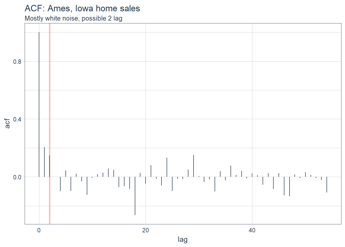
LSTM_train %>%
tidy_pacf(value, lags = 0:max_lag) %>%
ggplot(aes(lag, pacf)) +
geom_segment(aes(xend = lag, yend = 0), color = palette_light()[[1]]) +
# geom_vline(xintercept = 3, size = 1, color = palette_light()[[2]],alpha = 0.3) +
# annotate("text", label = "10 Year Mark", x = 130, y = 0.8,
# color = palette_light()[[2]], size = 6, hjust = 0) +
theme_tq() +
labs(title = "PACF: Ames, Iowa home sales",subtitle = 'Mostly white noise, possible 2 lag')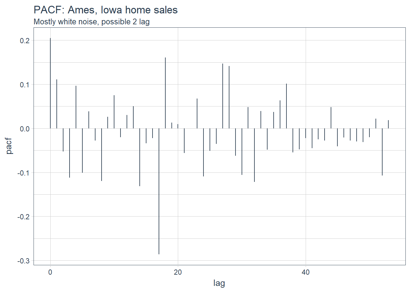
To remain completely objective here we can consult the forecast package:
forecast::auto.arima(LSTM_train$value,max.q = 0)## Series: LSTM_train$value
## ARIMA(1,0,0) with non-zero mean
##
## Coefficients:
## ar1 mean
## 0.2717 179891.444
## s.e. 0.1504 3282.577
##
## sigma^2 estimated as 3.3e+08: log likelihood=-616.46
## AIC=1238.92 AICc=1239.39 BIC=1244.94For the sake of exploration we can try the ar 2 framework
LSTM_train %>%
    tidy_acf(value, lags = 0:15) %>%
    ggplot(aes(lag, acf)) +
    geom_vline(xintercept = 2, size = 3, color = palette_light()[[2]],alpha=0.3) +
    geom_segment(aes(xend = lag, yend = 0), color = palette_light()[[1]]) +
    geom_point(color = palette_light()[[1]], size = 2) +
    geom_label(aes(label = acf %>% round(2)), vjust = -1,
              color = palette_light()[[1]]) +
    annotate("text", label = "2 Month Mark", x = 3, y = 0.8,
             color = palette_light()[[2]], size = 5, hjust = 0) +
    theme_tq() +
    labs(title = "ACF: Iowa",
         subtitle = "Zoomed in on Lags 1 to 15")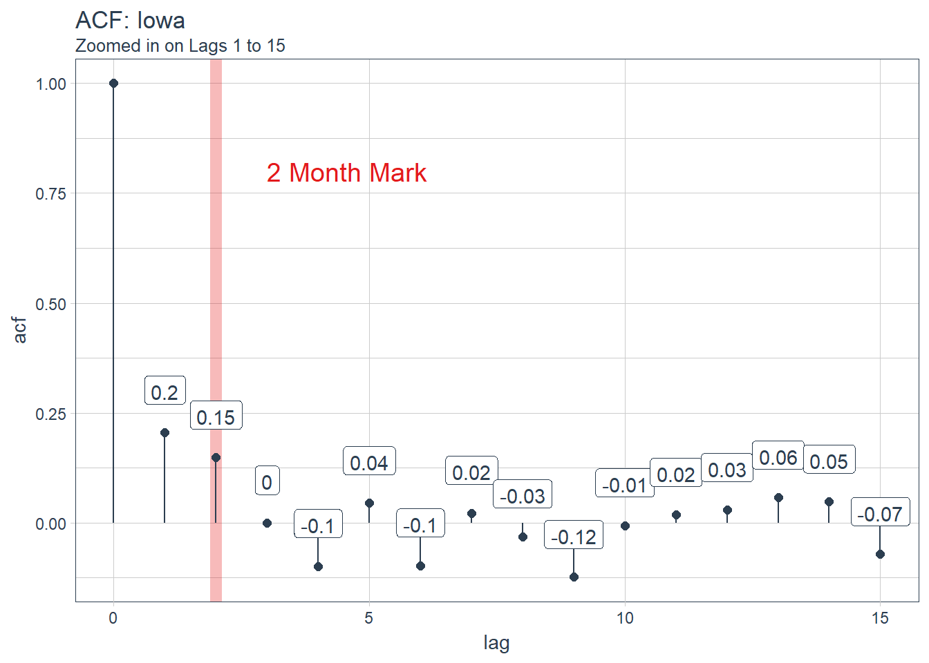
optimal_lag_setting <- 2For us to validate the model we will use a method called backtesting. Backtesting is basically splitting the data into different splits of data and for each split leaving out a future horizon that you can predict and measure accuracy. By testing all the different folds we can feel more certain of model performance since it wasn’t just a one time lucky score.
# periods_train <- 12 * 50
# periods_test  <- 12 * 10
# skip_span     <- 12 * 20

periods_train <- 36
periods_test  <- 3
skip_span     <- 6

rolling_origin_resamples <- rolling_origin(
    LSTM_train,
    initial    = periods_train,
    assess     = periods_test,
    cumulative = FALSE,
    skip       = skip_span
)

rolling_origin_resamples
## # Rolling origin forecast resampling
## # A tibble: 3 x 2
## splits id
## <list> <chr>
## 1 <S3: rsplit> Slice1
## 2 <S3: rsplit> Slice2
## 3 <S3: rsplit> Slice3A function that visualizes the different times series splits:
# Plotting function for a single split
plot_split <- function(split, expand_y_axis = TRUE, alpha = 1, size = 1, base_size = 14) {

    # Manipulate data
    train_tbl <- training(split) %>%
        add_column(key = "training")

    test_tbl  <- testing(split) %>%
        add_column(key = "testing")

    data_manipulated <- bind_rows(train_tbl, test_tbl) %>%
        as_tbl_time(index = index) %>%
        mutate(key = fct_relevel(key, "training", "testing"))

    # Collect attributes
    train_time_summary <- train_tbl %>%
        tk_index() %>%
        tk_get_timeseries_summary()

    test_time_summary <- test_tbl %>%
        tk_index() %>%
        tk_get_timeseries_summary()

    # Visualize
    g <- data_manipulated %>%
        ggplot(aes(x = index, y = value, color = key)) +
        geom_line(size = size, alpha = alpha) +
        theme_tq(base_size = base_size) +
        scale_color_tq() +
        labs(
            title    = glue("Split: {split$id}"),
            subtitle = glue("{train_time_summary$start} to {test_time_summary$end}"),
            y = "", x = ""
        ) +
        theme(legend.position = "none")

    if (expand_y_axis) {

        sun_spots_time_summary <- sun_spots %>%
            tk_index() %>%
            tk_get_timeseries_summary()

        g <- g +
            scale_x_date(limits = c(sun_spots_time_summary$start,
                                    sun_spots_time_summary$end))
    }

    return(g)
}
Plotting function that we can map over all these splits
# Plotting function that scales to all splits
plot_sampling_plan <- function(sampling_tbl, expand_y_axis = TRUE,
                               ncol = 3, alpha = 1, size = 1, base_size = 14,
                               title = "Sampling Plan") {

    # Map plot_split() to sampling_tbl
    sampling_tbl_with_plots <- sampling_tbl %>%
        mutate(gg_plots = map(splits, plot_split,
                              expand_y_axis = expand_y_axis,
                              alpha = alpha, base_size = base_size))

    # Make plots with cowplot
    plot_list <- sampling_tbl_with_plots$gg_plots

    p_temp <- plot_list[[1]] + theme(legend.position = "bottom")
    legend <- get_legend(p_temp)

    p_body  <- plot_grid(plotlist = plot_list, ncol = ncol)

    p_title <- ggdraw() +
        draw_label(title, size = 18, fontface = "bold", colour = palette_light()[[1]])

    g <- plot_grid(p_title, p_body, legend, ncol = 1, rel_heights = c(0.05, 1, 0.05))

    return(g)

}
Let’s visualize our backtesting folds:
rolling_origin_resamples %>%
    plot_sampling_plan(expand_y_axis = FALSE, ncol = 3, alpha = 1, size = 1, base_size = 10,
                       title = "Backtesting Strategy: Rolling Origin Sampling Plan")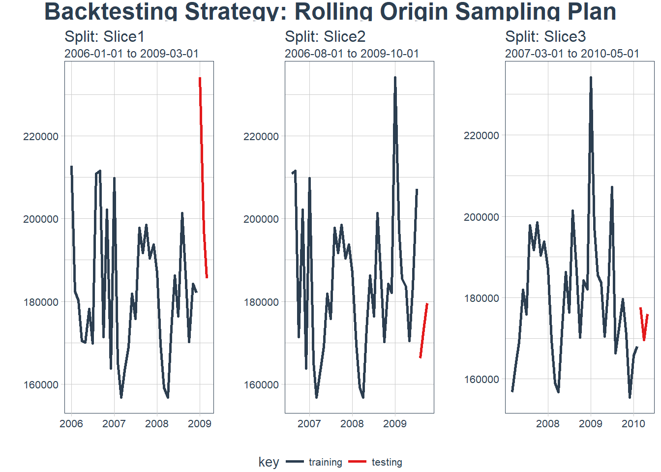
Test a LSTM model
OK, so now that we have a backtesting strategy set we should try to fit a model on one of the folds:
split    <- rolling_origin_resamples$splits[[1]]
split_id <- rolling_origin_resamples$id[[1]]

plot_split(split, expand_y_axis = FALSE, size = 0.5) +
    theme(legend.position = "bottom") +
    ggtitle(glue("Split: {split_id}"))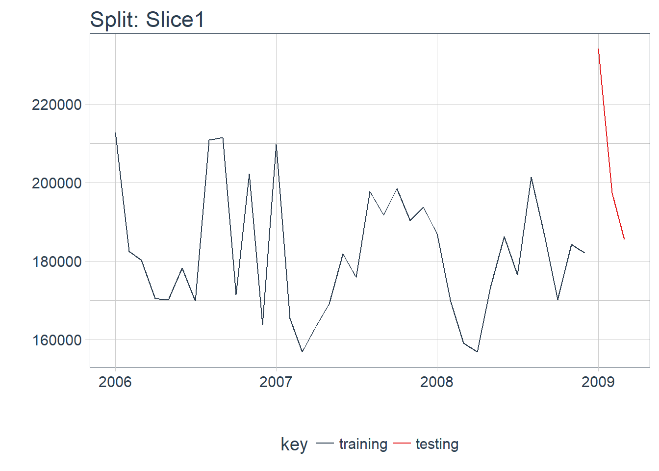
Split test/train
df_trn <- training(split)
df_tst <- testing(split)

df <- bind_rows(
    df_trn %>% add_column(key = "training"),
    df_tst %>% add_column(key = "testing")
) %>%
    as_tbl_time(index = index)

df
## # A time tibble: 39 x 3
## # Index: index
## index value key
## <date> <dbl> <chr>
## 1 2006-01-01 212711. training
## 2 2006-02-01 182493. training
## 3 2006-03-01 180162. training
## 4 2006-04-01 170443. training
## 5 2006-05-01 170079. training
## 6 2006-06-01 178162. training
## 7 2006-07-01 169873. training
## 8 2006-08-01 210880. training
## 9 2006-09-01 211548. training
## 10 2006-10-01 171406. training
## # ... with 29 more rowsScale and center the data
We can process this data using the recipes package
rec_obj <- recipe(value ~ ., df) %>%
    step_sqrt(value) %>%
    step_center(value) %>%
    step_scale(value) %>%
    prep()

df_processed_tbl <- bake(rec_obj, df)

df_processed_tbl
## # A tibble: 39 x 3
## index value key
## <date> <dbl> <fct>
## 1 2006-01-01 1.62 training
## 2 2006-02-01 -0.0515 training
## 3 2006-03-01 -0.186 training
## 4 2006-04-01 -0.757 training
## 5 2006-05-01 -0.778 training
## 6 2006-06-01 -0.302 training
## 7 2006-07-01 -0.791 training
## 8 2006-08-01 1.52 training
## 9 2006-09-01 1.56 training
## 10 2006-10-01 -0.699 training
## # ... with 29 more rowsWe will need to save the scaling factors so that we can restore the scale at the end
center_history <- rec_obj$steps[[2]]$means["value"]
scale_history  <- rec_obj$steps[[3]]$sds["value"]

c("center" = center_history, "scale" = scale_history)
## center.value scale.value
## 428.24106 20.34574Let’s define our model inputs:
# Model inputs
lag_setting  <- 3 # = nrow(df_tst)
batch_size   <- 3
train_length <- 24 # nrow(df_trn)
tsteps       <- 1
epochs       <- 300
Set up training and test sets
# Training Set
lag_train_tbl <- df_processed_tbl %>%
    mutate(value_lag = lag(value, n = lag_setting)) %>%
    filter(!is.na(value_lag)) %>%
    filter(key == "training") %>%
    tail(train_length)

x_train_vec <- lag_train_tbl$value_lag
x_train_arr <- array(data = x_train_vec, dim = c(length(x_train_vec), 1, 1))

y_train_vec <- lag_train_tbl$value
y_train_arr <- array(data = y_train_vec, dim = c(length(y_train_vec), 1))

# Testing Set
lag_test_tbl <- df_processed_tbl %>%
    mutate(
        value_lag = lag(value, n = lag_setting)
    ) %>%
    filter(!is.na(value_lag)) %>%
    filter(key == "testing")

x_test_vec <- lag_test_tbl$value_lag
x_test_arr <- array(data = x_test_vec, dim = c(length(x_test_vec), 1, 1))

y_test_vec <- lag_test_tbl$value
y_test_arr <- array(data = y_test_vec, dim = c(length(y_test_vec), 1))
Test a LSTM network to get a feel for the model:
model <- keras_model_sequential()

model %>%
    layer_lstm(units            = 10,
               input_shape      = c(tsteps, 1),
               batch_size       = batch_size,
               return_sequences = TRUE,
               stateful         = TRUE) %>%
    layer_lstm(units            = 10,
               return_sequences = FALSE,
               stateful         = TRUE) %>%
    layer_dense(units = 1)

model %>%
    compile(loss = 'mae', optimizer = 'adam')

model
## Model
## ___________________________________________________________________________
## Layer (type) Output Shape Param #
## ===========================================================================
## lstm_1 (LSTM) (3, 1, 10) 480
## ___________________________________________________________________________
## lstm_2 (LSTM) (3, 10) 840
## ___________________________________________________________________________
## dense_23 (Dense) (3, 1) 11
## ===========================================================================
## Total params: 1,331
## Trainable params: 1,331
## Non-trainable params: 0
## ___________________________________________________________________________for (i in 1:epochs) {
model %>% keras::fit(x = x_train_arr,
y = y_train_arr,
batch_size = batch_size,
epochs = 1,
verbose = 0,
shuffle = FALSE)
model %>% reset_states()
# cat("Epoch: ", i, '\n')
}Now let’s predict the next 3 months so we can test the performance of the model
pred_out <- model %>%
    predict(x_test_arr, batch_size = batch_size) %>%
    .[,1]

# Retransform values
pred_tbl <- tibble(
    index   = lag_test_tbl$index,
    value   = (pred_out * scale_history + center_history)^2
)

# Combine actual data with predictions
tbl_1 <- df_trn %>%
    add_column(key = "actual")

tbl_2 <- df_tst %>%
    add_column(key = "actual")

tbl_3 <- pred_tbl %>%
    add_column(key = "predict")

# Create time_bind_rows() to solve dplyr issue
time_bind_rows <- function(data_1, data_2, index) {
    index_expr <- enquo(index)
    bind_rows(data_1, data_2) %>%
        as_tbl_time(index = !! index_expr)
}

ret <- list(tbl_1, tbl_2, tbl_3) %>%
    reduce(time_bind_rows, index = index) %>%
    arrange(key, index) %>%
    mutate(key = as_factor(key))

ret
## # A time tibble: 42 x 3
## # Index: index
## index value key
## <date> <dbl> <fct>
## 1 2006-01-01 212711. actual
## 2 2006-02-01 182493. actual
## 3 2006-03-01 180162. actual
## 4 2006-04-01 170443. actual
## 5 2006-05-01 170079. actual
## 6 2006-06-01 178162. actual
## 7 2006-07-01 169873. actual
## 8 2006-08-01 210880. actual
## 9 2006-09-01 211548. actual
## 10 2006-10-01 171406. actual
## # ... with 32 more rowsFunction to calculate rmse for us
calc_rmse <- function(prediction_tbl) {

    rmse_calculation <- function(data) {
        data %>%
            spread(key = key, value = value) %>%
            select(-index) %>%
            filter(!is.na(predict)) %>%
            rename(
                truth    = actual,
                estimate = predict
            ) %>%
            rmse(truth, estimate)
    }

    safe_rmse <- possibly(rmse_calculation, otherwise = NA)

    safe_rmse(prediction_tbl)

}
which is:
calc_rmse(ret) ## [1] 32301.01Function that plots the errors…
# Setup single plot function
plot_prediction <- function(data, id, alpha = 1, size = 2, base_size = 14) {

    rmse_val <- calc_rmse(data)

    g <- data %>%
        ggplot(aes(index, value, color = key)) +
        geom_point(alpha = alpha, size = size) +
        # geom_line(alpha = alpha, size = size)+
        theme_tq(base_size = base_size) +
        scale_color_tq() +
        theme(legend.position = "none") +
        labs(
            title = glue("{id}, RMSE: {round(rmse_val, digits = 1)}"),
            x = "", y = ""
        )

    return(g)
}
Let’s see the performance:
ret %>%
    plot_prediction(id = split_id, alpha = 0.65) +
    theme(legend.position = "bottom")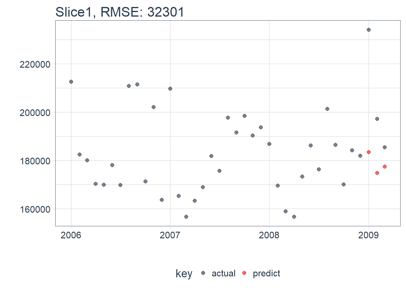
Awesome the LSTM model is ready to start making us some predictions!
Now we need to back test the model on all the time slices now since we now have a method we can map over all of them simultaneously
Everything set… time to get started!

Back test LSTM model
Let’s create a function that will compile, fit and predict the LSTM network.
Basically this function will do everything we just did for testing the single fold so we can map it accross all the folds
predict_keras_lstm <- function(split, epochs = 300, lag_setting, batch_size, train_length,  tsteps, optimizer = 'adam',...) {

    lstm_prediction <- function(split, epochs, lag_setting, batch_size, train_length,  tsteps, optimizer, ...) {

        # 5.1.2 Data Setup
        df_trn <- training(split)
        df_tst <- testing(split)

        df <- bind_rows(
            df_trn %>% add_column(key = "training"),
            df_tst %>% add_column(key = "testing")
        ) %>%
            as_tbl_time(index = index)

        # 5.1.3 Preprocessing
        rec_obj <- recipe(value ~ ., df) %>%
            step_sqrt(value) %>%
            step_center(value) %>%
            step_scale(value) %>%
            prep()

        df_processed_tbl <- bake(rec_obj, df)

        center_history <- rec_obj$steps[[2]]$means["value"]
        scale_history  <- rec_obj$steps[[3]]$sds["value"]

        # # 5.1.4 LSTM Plan
        # lag_setting  <- 120 # = nrow(df_tst)
        # batch_size   <- 40
        # train_length <- 440
        # tsteps       <- 1
        # epochs       <- epochs

        # 5.1.5 Train/Test Setup
        lag_train_tbl <- df_processed_tbl %>%
            mutate(value_lag = lag(value, n = lag_setting)) %>%
            filter(!is.na(value_lag)) %>%
            filter(key == "training") %>%
            tail(train_length)

        x_train_vec <- lag_train_tbl$value_lag
        x_train_arr <- array(data = x_train_vec, dim = c(length(x_train_vec), 1, 1))

        y_train_vec <- lag_train_tbl$value
        y_train_arr <- array(data = y_train_vec, dim = c(length(y_train_vec), 1))

        lag_test_tbl <- df_processed_tbl %>%
            mutate(
                value_lag = lag(value, n = lag_setting)
            ) %>%
            filter(!is.na(value_lag)) %>%
            filter(key == "testing")

        x_test_vec <- lag_test_tbl$value_lag
        x_test_arr <- array(data = x_test_vec, dim = c(length(x_test_vec), 1, 1))

        y_test_vec <- lag_test_tbl$value
        y_test_arr <- array(data = y_test_vec, dim = c(length(y_test_vec), 1))

        # 5.1.6 LSTM Model
        model <- keras_model_sequential()

        model %>%
            layer_lstm(units            = 10,
                       input_shape      = c(tsteps, 1),
                       batch_size       = batch_size,
                       return_sequences = TRUE,
                       stateful         = TRUE) %>%
            layer_lstm(units            = 10,
                       return_sequences = FALSE,
                       stateful         = TRUE) %>%
            layer_dense(units = 1)

        model %>%
            compile(loss = 'mae', optimizer = optimizer)

        # 5.1.7 Fitting LSTM
        for (i in 1:epochs) {
            model %>% fit(x          = x_train_arr,
                          y          = y_train_arr,
                          batch_size = batch_size,
                          epochs     = 1,
                          verbose    = 0,
                          shuffle    = FALSE)

            model %>% reset_states()
            # cat("Epoch: ", i, '\n')

        }

        # 5.1.8 Predict and Return Tidy Data
        # Make Predictions
        pred_out <- model %>%
            predict(x_test_arr, batch_size = batch_size) %>%
            .[,1]

        # Retransform values
        pred_tbl <- tibble(
            index   = lag_test_tbl$index,
            value   = (pred_out * scale_history + center_history)^2
        )

        # Combine actual data with predictions
        tbl_1 <- df_trn %>%
            add_column(key = "actual")

        tbl_2 <- df_tst %>%
            add_column(key = "actual")

        tbl_3 <- pred_tbl %>%
            add_column(key = "predict")

        # Create time_bind_rows() to solve dplyr issue
        time_bind_rows <- function(data_1, data_2, index) {
            index_expr <- enquo(index)
            bind_rows(data_1, data_2) %>%
                as_tbl_time(index = !! index_expr)
        }

        ret <- list(tbl_1, tbl_2, tbl_3) %>%
            reduce(time_bind_rows, index = index) %>%
            arrange(key, index) %>%
            mutate(key = as_factor(key))

        return(ret)

    }

    safe_lstm <- possibly(lstm_prediction, otherwise = NA)

    safe_lstm(split, epochs, lag_setting, batch_size, train_length,  tsteps, optimizer, ...)

}
Set our test parameters (remember that the training samples must be divisable by the batch size)
lag_setting  <- 3 # = nrow(df_tst)
batch_size   <- 3
train_length <- 24 # nrow(df_trn)
tsteps       <- 1
epochs       <- 300
Now we map the LSTM model over all our times series folds to back test:
sample_predictions_lstm_tbl <-
rolling_origin_resamples %>%
    mutate(predict = map(
        splits,
        predict_keras_lstm,
        epochs = 300,
        lag_setting = lag_setting,
        batch_size = batch_size,
        train_length = train_length ,
        tsteps = tsteps ,
        optimizer = 'adam'
        ))

sample_predictions_lstm_tbl %>% head
The same way we created a funtion to plot the test and training sets we can make one to plot the actuals and predicted values:
plot_predictions <- function(sampling_tbl, predictions_col,
                             ncol = 3, alpha = 1, size = 2, base_size = 14,
                             title = "Backtested Predictions") {

    predictions_col_expr <- enquo(predictions_col)

    # Map plot_split() to sampling_tbl
    sampling_tbl_with_plots <- sampling_tbl %>%
        mutate(gg_plots = map2(!! predictions_col_expr, id,
                               .f        = plot_prediction,
                               alpha     = alpha,
                               size      = size,
                               base_size = base_size))

    # Make plots with cowplot
    plot_list <- sampling_tbl_with_plots$gg_plots

    p_temp <- plot_list[[1]] + theme(legend.position = "bottom")
    legend <- get_legend(p_temp)

    p_body  <- plot_grid(plotlist = plot_list, ncol = ncol)


    p_title <- ggdraw() +
        draw_label(title, size = 18, fontface = "bold", colour = palette_light()[[1]])

    g <- plot_grid(p_title, p_body, legend, ncol = 1, rel_heights = c(0.05, 1, 0.05))

    return(g)

}
Let’s see how our LSTM model did:
sample_predictions_lstm_tbl %>%
    plot_predictions(predictions_col = predict, alpha = 0.5, size = 1, base_size = 10,
                     title = "Keras Stateful LSTM: Backtested Predictions")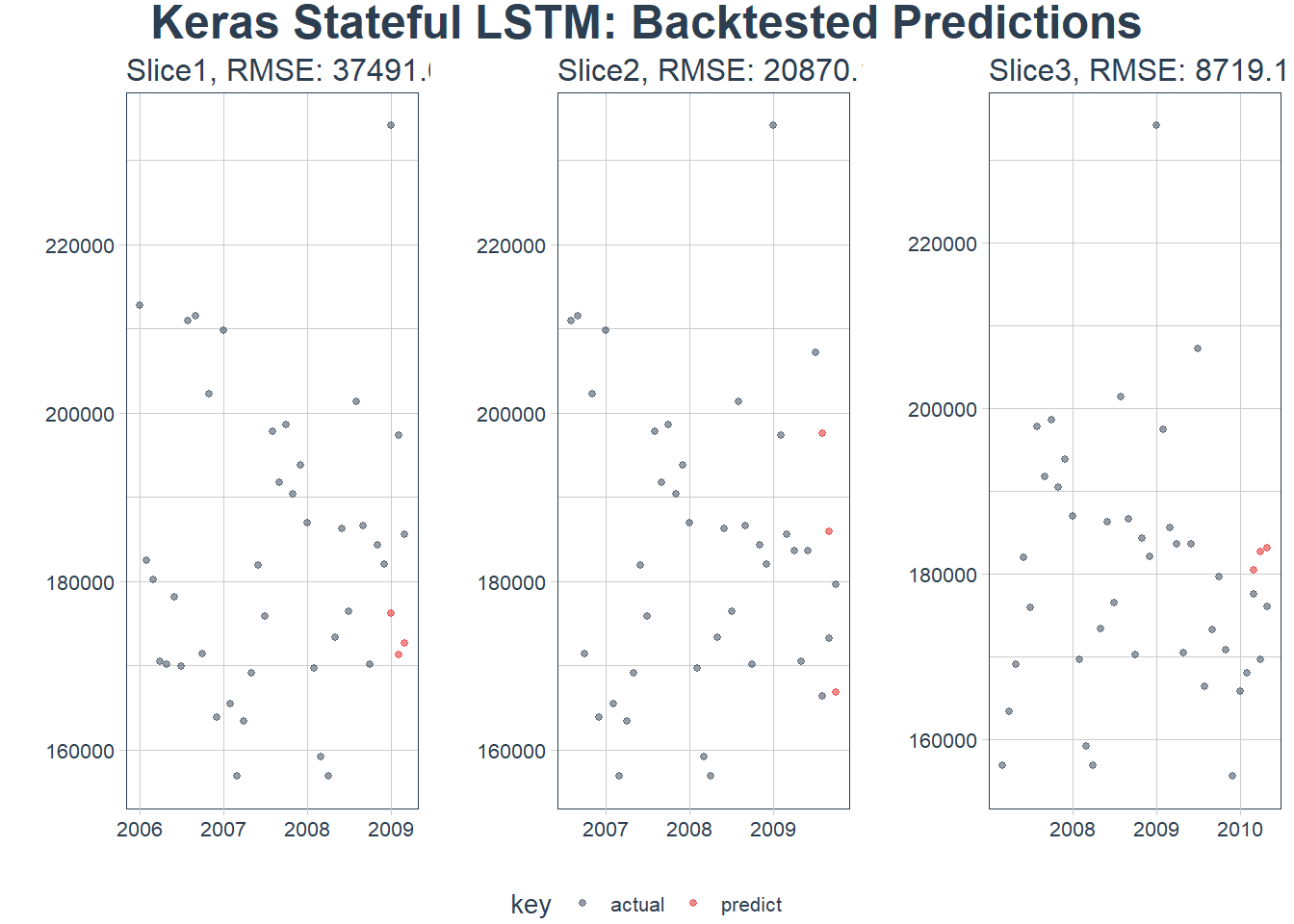
Seems to be working! Even though we had small correlations
We can reuse our rmse calculator to see our accuracy over each time slice:
sample_rmse_tbl <- sample_predictions_lstm_tbl %>%
    mutate(rmse = map_dbl(predict, calc_rmse)) %>%
    select(id, rmse)

sample_rmse_tbl
## # Rolling origin forecast resampling
## # A tibble: 3 x 2
## id rmse
## * <chr> <dbl>
## 1 Slice1 37492.
## 2 Slice2 20870.
## 3 Slice3 8719.We can plot the RMSE over the various folds:
sample_rmse_tbl %>%
    ggplot(aes(rmse)) +
    geom_histogram(aes(y = ..density..), fill = palette_light()[[1]], bins = 5) +
    geom_density(fill = palette_light()[[1]], alpha = 0.5) +
    theme_tq() +
    ggtitle("Histogram of RMSE")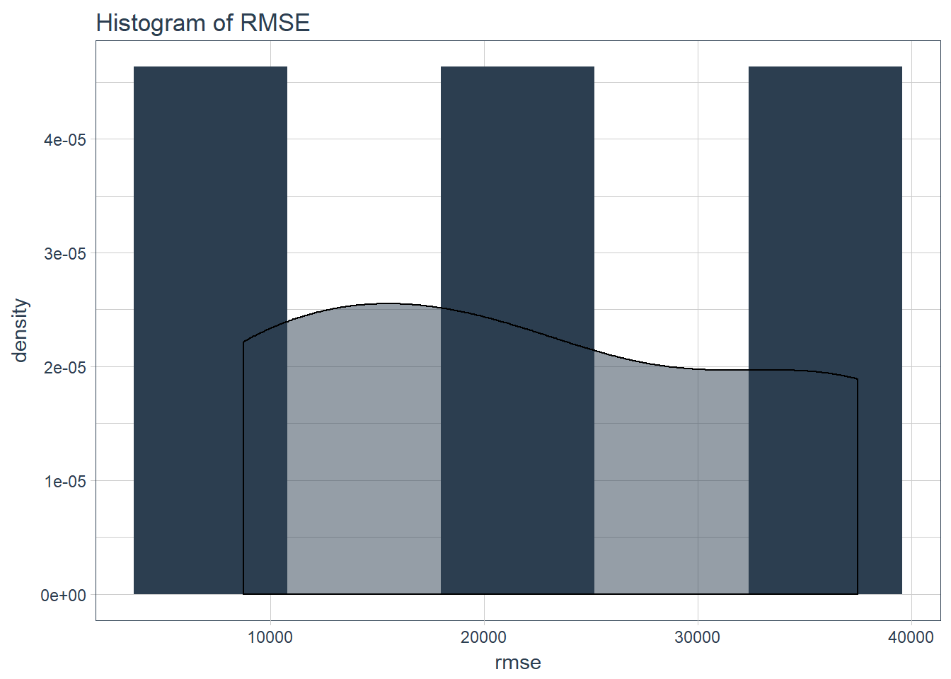
And the distribution is:
sample_rmse_tbl %>%
    summarize(
        mean_rmse = mean(rmse),
        sd_rmse   = sd(rmse)
    )
## # Rolling origin forecast resampling
## # A tibble: 1 x 2
## mean_rmse sd_rmse
## <dbl> <dbl>
## 1 22360. 14444.Test final model on full dataset
Now we create our function that will test the LSTM model on all the data:
predict_keras_lstm_future <- function(data, epochs = 300,lag_setting, batch_size, train_length,  tsteps, optimizer = 'adam',...) {

    lstm_prediction <- function(data, epochs,lag_setting, batch_size, train_length,  tsteps, optimizer, ...) {

        # 5.1.2 Data Setup (MODIFIED)
        df <- data

        # 5.1.3 Preprocessing
        rec_obj <- recipe(value ~ ., df) %>%
            step_sqrt(value) %>%
            step_center(value) %>%
            step_scale(value) %>%
            prep()

        df_processed_tbl <- bake(rec_obj, df)

        center_history <- rec_obj$steps[[2]]$means["value"]
        scale_history  <- rec_obj$steps[[3]]$sds["value"]

        # 5.1.5 Train Setup (MODIFIED)
        lag_train_tbl <- df_processed_tbl %>%
            mutate(value_lag = lag(value, n = lag_setting)) %>%
            filter(!is.na(value_lag)) %>%
            tail(train_length)

        x_train_vec <- lag_train_tbl$value_lag
        x_train_arr <- array(data = x_train_vec, dim = c(length(x_train_vec), 1, 1))

        y_train_vec <- lag_train_tbl$value
        y_train_arr <- array(data = y_train_vec, dim = c(length(y_train_vec), 1))

        x_test_vec <- y_train_vec %>% tail(lag_setting)
        x_test_arr <- array(data = x_test_vec, dim = c(length(x_test_vec), 1, 1))

        # 5.1.6 LSTM Model
        model <- keras_model_sequential()

        model %>%
            layer_lstm(units            = 10,
                       input_shape      = c(tsteps, 1),
                       batch_size       = batch_size,
                       return_sequences = TRUE,
                       stateful         = TRUE) %>%
            layer_lstm(units            = 10,
                       return_sequences = FALSE,
                       stateful         = TRUE) %>%
            layer_dense(units = 1)

        model %>%
            compile(loss = 'mae', optimizer = optimizer)

        # 5.1.7 Fitting LSTM
        for (i in 1:epochs) {
            model %>% fit(x          = x_train_arr,
                          y          = y_train_arr,
                          batch_size = batch_size,
                          epochs     = 1,
                          verbose    = 0,
                          shuffle    = FALSE)

            model %>% reset_states()
            # cat("Epoch: ", i, '\n')

        }

        # 5.1.8 Predict and Return Tidy Data (MODIFIED)
        # Make Predictions
        pred_out <- model %>%
            predict(x_test_arr, batch_size = batch_size) %>%
            .[,1]

        # Make future index using tk_make_future_timeseries()
        idx <- data %>%
            tk_index() %>%
            tk_make_future_timeseries(n_future = lag_setting)

        # Retransform values
        pred_tbl <- tibble(
            index   = idx,
            value   = (pred_out * scale_history + center_history)^2
        )

        # Combine actual data with predictions
        tbl_1 <- df %>%
            add_column(key = "actual")

        tbl_3 <- pred_tbl %>%
            add_column(key = "predict")

        # Create time_bind_rows() to solve dplyr issue
        time_bind_rows <- function(data_1, data_2, index) {
            index_expr <- enquo(index)
            bind_rows(data_1, data_2) %>%
                as_tbl_time(index = !! index_expr)
        }

        ret <- list(tbl_1, tbl_3) %>%
            reduce(time_bind_rows, index = index) %>%
            arrange(key, index) %>%
            mutate(key = as_factor(key))

        return(ret)

    }

    safe_lstm <- possibly(lstm_prediction, otherwise = NA)

    safe_lstm(data, epochs, lag_setting, batch_size, train_length,  tsteps, optimizer, ...)

}
future_LSTM_tbl <-
predict_keras_lstm_future(LSTM_train,
epochs = 300,
lag_setting = lag_setting,
batch_size = batch_size,
train_length = train_length ,
tsteps = tsteps ,
optimizer = 'adam'
)future_LSTM_tbl %>%
# filter_time("2008" ~ "end") %>%
plot_prediction(id = NULL, alpha = 0.4, size = 1.5) +
theme(legend.position = "bottom") +
ggtitle("House prices: 3 Month Forecast using LSTM deep neural net", subtitle = "Using the full dataset")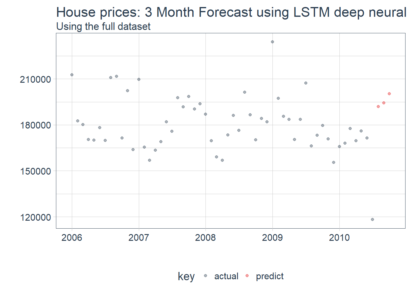
Combine LSTM and Inference networks into 1 deep neural network??
I was tempted to combine these 2 networks together so that I could backpropegate them simultaneously. This would allow us to use the inference network using descriptive features together with the macro economic trends in the market of housing prices.
To stack different deep neural networks together we can use the keras API like this:
Define complete model
# data.frame(factor = 1:100,res = 2324/1:100) %>% filter(res == trunc(res))
# batch_size <- 28
batch_size <- 83

inference_input <-
layer_input( name = "inference_input",batch_shape = c(batch_size,265))

encoded_inference_network <-
inference_input %>%
layer_dense(units = 128, activation = 'relu') %>% # 1 axis and nr features = number columns
layer_batch_normalization() %>%
# layer_dropout(rate = 0.2) %>%
layer_dense(units = 64, activation ='relu') %>%
layer_dense(units = 32, activation ='relu')
# layer_dense(units = 25, activation ='relu') %>%

LSTM_input <-
layer_input(name = "LSTM_input",batch_shape = c(batch_size,1,1))

encoded_LSTM_network <-
LSTM_input %>%
            layer_lstm(units            = 100,
                       batch_size       = batch_size,
                       return_sequences = TRUE,
                       stateful         = TRUE) %>%
            layer_lstm(units            = 100,
                       return_sequences = FALSE,
                       stateful         = TRUE)

concatenated <-
layer_concatenate(list(encoded_LSTM_network, encoded_inference_network))

house_price <- concatenated %>%
layer_dense(units = 5, activation = "relu") %>%
layer_dense(units = 1)

model <- keras_model(list(LSTM_input, inference_input), house_price)
model %>% compile(
optimizer = "adam",
loss='mse',
metrics = c('mae')
)
Create our LSTM input:
I realised very quickly that we have a small problem here… To backpropogate both networks simultaneously they would need to feed the same batch of inputs into both networks! But our LSTM model was trained on monthly data - this means I had a 1 to many relationship between the 2 models inputs.
I tried to naively circumvent this by infering the lag of prices on a per house level. We could do this by simply using the average shift and applying it as a predicted lag index:
prepare_LSTM_input <- function(monthly_ts,sample_ts,lag_setting,train_length) {

# 5.1.5 Train Setup (MODIFIED)
lag_train_tbl <- monthly_ts %>%
    mutate(value_lag_month = lag(value, n = lag_setting)) %>%
    filter(!is.na(value_lag_month)) %>%
    tail(train_length) %>%
rename(value_month = value)

join_df <-
sample_ts %>%
left_join(lag_train_tbl, by = 'index') %>%
mutate(value_lag = value * value_lag_month/value_month) %>%
select(index,value,value_lag)

rec_obj <- recipe(index ~ ., join_df) %>%
    step_sqrt(all_predictors()) %>%
    step_center(all_predictors()) %>%
    step_scale(all_predictors()) %>%
    prep()

df_processed_tbl <- bake(rec_obj, join_df)

center_history <- rec_obj$steps[[2]]$means["value"]
scale_history  <- rec_obj$steps[[3]]$sds["value"]

x_train_vec <- df_processed_tbl$value_lag
x_train_arr <- array(data = x_train_vec, dim = c(length(x_train_vec), 1, 1))

y_train_vec <- df_processed_tbl$value
y_train_arr <- array(data = y_train_vec, dim = c(length(y_train_vec), 1))

return(list(LSTM_input = x_train_arr, LSTM_target = y_train_arr, center_history = center_history, scale_history = scale_history))
}

return_original_scale <- function(pred_out, scale_history,center_history) {
return((pred_out * scale_history + center_history)^2)
}
sample_ts <- train %>%
select(SalePrice,Yr.Sold,Mo.Sold) %>%
tidyr::unite(col = index,Yr.Sold,Mo.Sold,sep="-") %>%
mutate(index = index %>% zoo::as.yearmon() %>% as_date()) %>%
rename(value = SalePrice) %>% as_tbl_time(index = index)
LSTM_input_full_model <-
prepare_LSTM_input(monthly_ts = LSTM_train,sample_ts = sample_ts,lag_setting = 3,train_length = 24)So let’s try to train the 2 deep neural networks simulteneously:
history <- model %>% fit(
list(inference_input = inference_train_X,
LSTM_input = LSTM_input_full_model$LSTM_input),
LSTM_input_full_model$LSTM_target,
epochs = 300,
batch_size = batch_size,
shuffle = FALSE
,verbose = 0
)
The network can’t back propogate properly! This is because the LSTM model needs the inputs to move consistently through time. Even though our inputs are correctly lagged we have inconsistent numbers of rows for each time index which ruins the ‘memory’ part of the model…
What we can do however is use the prediction of price movement as a feature in the inference model. We can train the inference model by adding the future average price of properties by month by region truncating that data that has no future observations.
Then we train the LSTM and inference networks seperately - the LSTM then predicts that future movement for us so we can test the accuracy of our combined model feeding the LSTM into the inference network into a result
Future additions
I will build this feed forward from LSTM to inference network soon and then update this post!! Watch this space!!