Important Predictors of Spend Behaviour

Anri
Sep 9, 2021 in GENERAL
modelling

Introduction:

A retailer wishes to understand a variety of shopping behaviour at its stores. For example how does its existing customers compare to its new customers? What about its lost customers compared to its existing customers? Does its customers look different from its competitors? To answer these questions we had a look at establishing which customer characteristics are the most important when categorising customers into the above spend behaviour groups.

The Model Components:

We made use of the Machine Learning technique: Random Forest Modelling of Classification Trees. The response being a binary field where a customer can fall into one of two categories per model:

New Customers vs Lost Customers
New vs Existing Customers
Lost vs Existing Customers
High vs Low Share of Wallet(SoW) Customers
Increasing vs Decreasing Share of Wallet (SoW) Customers
Top vs Bottom Spend per Month (SPM) Customers
Increasing vs Decreasing Spend per Month(SPM) Customers
My Customers vs Competitor Customers

Some helpful definitions:

New Customer: They shopped at the Retailer within the given Spend Category for the first time in 2020
Existing Customer: Shopped at Retailer Spend Category in 2018,2019 and 2020
Lost Customer: Shopped at Retailer Spend Category in 2018, 2019 but not in 2020 or 2021

The predictors in the models consisted of a range of customer characteristics:

Demographics
Credit Behaviour
Affluency
Broader Industry Spend Behaviour
Spend Behaviour at Retailer and immediate competitors

Technical Modelling Summary

Samples and field preperation

A sample of ~1 million customers was taken for each model, with 500k belonging to each of the two response groups
All predictor fields were cleaned before loading into R (Though this could have been done in R as well)
Missing values were imputed for derived income and age
Missing credit information was conservatively set to 0
Any ratios consisting of missing credit information were also set to zero
All categorical fields are transformed to factor variables

The Model Run & Fit

A model was fit for each Retailer-Spend Category combination for a given resposnse of interest(1-8 listed above)
Each model had a total of 500 trees built on a training set consisting of 80% of the observations, with 20% held out as a test set
At each split in the Classification tree only a subset of the available predictors is considered (the square root of the number of predictors) This is to ensure that not only the most dominant variables are considered
The Goodness of Fit of the model is assessed based on the proportion of correctly classified customers in the test set
Variable Importance is recorded as the mean decrease in the Gini Coefficent. The Gini Coefficient being the probabilty of incorrectly classifying an individual to the wrong resonse category.
The algorithm is run in parallel across 7 cores

Model Output

We pull out the most important predictors per predictor category (Demographics, Credit Behaviour etc) based on the mean deacrease in the Gini Coefficient as a result of including that variable in the model
We then calculate the average value / most prominant level of that predictor across the response groups to understand how the response groups differ for this predictor variable

Sample Code

Here we run through the modelling process for the My Customer vs Competitor Customers model on a smaller sample of 50k customers.

Data Load & Analysis Prep

#################################
#Script Libraries
#################################
rm(list = ls())
start_time <- Sys.time()

#analysis
library(dplyr)
library(randomForest)
#library(adabag)
#data loading
#library(DBI)
#library(RODBC)
#performance
#library(doParallel)
#library(foreach)
library(ggplot2)

#db<-odbcConnect( "sbsa_prod")
#con <- dbConnect(odbc::odbc(), "sbsa_prod", bigint="integer" )

# Script Variables
script_num <- 8

Responses <- c('New vs Lost Customers', 
               'New vs Existing Customers', 
               'Lost vs Existing Customers', 
               'High vs Low SoW', 
               'Increasing vs Decreasing SoW',
               'Top vs Bottom SPM Percentile',
               'Increasing vs Decreasing Spend',
               'My Customer vs Competitor Customers')


Retailer_Category <- list(c('R2','General M'), c('R2','Grocery'), c('R2','All'),
                          c('R1','General M'), c('R1','All'),
                          c('Competitors','General M'), c('Competitors','Grocery'), c('Competitors','All'))

regtree_input <- dbGetQuery(con, 'select * from sds.blog_MVP2reg_data;')
pred_categories <- dbGetQuery(con, 'select * from sds.mst_reg_pred_categories;')

saveRDS(regtree_input, file = 'imp_pred_spend_behav_data.RDS')

Fied Prep

Remove unnecessary fields
Convert all categorical fields to be factors
Handle missing values

#################################
# Data Cleaning
#################################

#field selection
regtree_data <- regtree_input %>% select(-c(age_bin,
                                            personal_loan_balance_bin,
                                            credit_card_balance_bin,
                                            home_loan_balance_bin, 
                                            vehicle_loan_balance_bin,
                                            credit_over_debit_spend_bin,
                                            prop_spend_credit_bin,
                                            prop_disposable_income_bin,
                                            prop_cash_bin,
                                            prop_spend_brand_low_bin,
                                            prop_spend_brand_medium_bin,
                                            prop_spend_brand_high_bin
))

rm(regtree_input)

#################################
# Field Prep
## Factor Variables
#################################

###########
# Response#
###########

regtree_data$response_ind <- factor(regtree_data$response_ind)


###############
# Demographics#
###############

## Province Area
## Gender
regtree_data$gender_id <- factor(regtree_data$gender_id)
#language
regtree_data$language_id <- factor(regtree_data$language_id)
## Ethnicity 
regtree_data$ethnicity_id <- factor(regtree_data$ethnicity_id)

## Marketing
regtree_data$receives_marketing_id <- factor(regtree_data$receives_marketing_id)
##segment code
regtree_data$segment_id <- factor(regtree_data$segment_id)
## Ucount Member
regtree_data$ucount_member_id <- factor(regtree_data$ucount_member_id)


############
# Affluency#
############
regtree_data$has_house <- factor(regtree_data$has_house)
regtree_data$has_home_loan <- factor(regtree_data$has_home_loan)
regtree_data$has_vehicle <- factor(regtree_data$has_vehicle)
regtree_data$has_vehicle_loan <- factor(regtree_data$has_vehicle_loan)
regtree_data$has_credit_card <- factor(regtree_data$has_credit_card)
regtree_data$has_personal_loan <- factor(regtree_data$has_personal_loan)
regtree_data$receives_regular_income <- factor(regtree_data$receives_regular_income)
regtree_data$HML_score_bin <- factor(regtree_data$HML_score_bin)
regtree_data$spend_indicator <- factor(regtree_data$spend_indicator)


###################
# Credit Behaviour#
###################
regtree_data$has_credit <- factor(regtree_data$has_credit)
regtree_data$has_unsecured_credit <- factor(regtree_data$has_unsecured_credit)
regtree_data$has_secured_credit <- factor(regtree_data$has_secured_credit)
regtree_data$income_drop_detected <- factor(regtree_data$income_drop_detected)


###########################
#Missing Values Imputation#
##########################

med_income <- median(regtree_data$derived_income, na.rm = TRUE)
regtree_data[is.na(regtree_data$derived_income),"derived_income"] <- med_income

regtree_data[is.na(regtree_data$avg_ATV),"avg_ATV"] <- 0
regtree_data[is.na(regtree_data$avg_SPM),"avg_SPM"] <- 0
regtree_data[is.na(regtree_data$avg_Freq),"avg_Freq"] <- 0

The Random Forest Model

############################################
############## RANDOM FOREST ###############
############################################

RF_model <- function(regtree_data,
                     Current_Response,
                     #Current_Period_Index,
                     Current_Retailer,
                     Current_Category,
                     model_performance_record,
                     variable_importance_record
)
{
  
  ##### (1.1) Input data #####
  regtree_input_data <- regtree_data %>% filter(response_metric == Current_Response &
                                                  #Period_Index == Current_Period_Index & 
                                                  Retailer == Current_Retailer & 
                                                  Category == Current_Category) %>%
    select(-c(response_metric,Retailer,Category,spend_indicator))
  ##### (1.2) Test and Training set ##### 
  
  ## test set
  test_ids <- sample(regtree_input_data$party_id,length(unique(regtree_input_data$party_id))/5)
  test_set <- regtree_input_data %>% filter(party_id %in% test_ids) %>% select(-c(party_id))
  xtest_set <- test_set %>% select(-response_ind)
  ytest_set <- test_set %>% select(response_ind)
  ytest_set$response_ind <- factor(ytest_set$response_ind)
  rm(test_set)
  

  ## training set
  training_set <- regtree_input_data %>% filter(!(party_id %in% test_ids)) %>% select(-c(party_id))

  
  ## variables
  num_vars <- sqrt(ncol(training_set) -1)
  
  
  ##### (2.1) RANDOM FOREST #####
  cl <- makeCluster(7)
  registerDoParallel(cl)
  randomForest_output <- foreach(ntree=rep(100, 5),
                                 .combine = combine, 
                                 .packages='randomForest') %dopar% randomForest(response_ind ~ ., 
                                                                                data=training_set, 
                                                                                xtest = xtest_set,
                                                                                ytest = ytest_set$response_ind,
                                                                                ntree = ntree, 
                                                                                replace = T,
                                                                                mtry = num_vars,
                                                                                #nodesize = 500, 
                                                                                #sampsize=27710,
                                                                                importance=TRUE#,
                                                                                #proximity=TRUE,
                                                                                #na.action=na.roughfix,
                                 ) 
  stopCluster(cl)
  
  ##### (2.2) RANDOM FOREST TEST PERFORMANCE #####
  
  ## Current Hit Record
  current_hit_record <- data.frame(actual = c(ytest_set))
  current_hit_record <- bind_cols(actual = current_hit_record,randomForest_output$test$predicted)
  colnames(current_hit_record) <- c('Actual', 'Predicted')
  current_hit_record <- current_hit_record %>% mutate(hit_status = if_else(Actual == Predicted,1,0))
  current_hit_rate <- sum(current_hit_record$hit_status)/nrow(current_hit_record)
  
  
  ##### (2.3) OOB Error #####
  
  ### Error Rate
  #OOB_error <- c(OOB_error,randomForest_output$err.rate)
  
  ### Confusion Matrix
  #confusion_matrix <- c(confusion_matrix,randomForest_output$confusion)
  
  
  ## Current Model Performance
  current_model_performance <- bind_cols(Response = Current_Response,
                                         #Period_Index = Current_Period_Index,
                                         Retailer = Current_Retailer,
                                         Category = Current_Category,
                                         hit_rate = current_hit_rate)
  
  
  ## Appending Current Performance
  model_performance_record <- bind_rows(model_performance_record,current_model_performance)
  
  
  
  ##### (3) VARIABLE IMPORTANCE #####
  
  ## Variable ranking
  variable_importance <- as.data.frame(round(importance(randomForest_output), 0)[,4])
  variable_importance <- bind_cols(variable_name = row.names(variable_importance),variable_importance)
  colnames(variable_importance) <- c('variable_name', 'variable_importance')
  
  variable_importance <- merge(x = variable_importance, y = pred_categories, by = c('variable_name'), all.x = TRUE)
  variable_importance <- variable_importance %>% arrange(desc(variable_importance)) %>% mutate(variable_rank = row_number())
  variable_importance <- variable_importance %>% group_by(pred_category) %>% arrange(desc(variable_importance)) %>% mutate(category_rank = row_number())
  
  ## Current Variable Importance Record
  current_variable_importance <- variable_importance %>% filter(category_rank <= 15)
  current_variable_importance <- bind_cols(Response = rep(Current_Response,nrow(current_variable_importance)),
                                           Retailer = rep(Current_Retailer,nrow(current_variable_importance)),
                                           Category = rep(Current_Category,nrow(current_variable_importance)),
                                           current_variable_importance)
  
  ## Appending Current Variable Importance to Record
  variable_importance_record <- bind_rows(variable_importance_record,current_variable_importance)
  
  return(list(variable_importance_record,model_performance_record))
}

Model Execution and Record

#################################
## Model Execution and Record ##
#################################

Current_Response <- Responses[script_num]

## model performance record
MyComp_Cust_model_performance_record <- data.frame()

## variable importance record
MyComp_Cust_variable_importance_record <- data.frame()


for (j in 1:length(Retailer_Category)) 
{
  Current_Retailer <- Retailer_Category[[j]][1]
  Current_Category <- Retailer_Category[[j]][2]
  
  
  RF_model_output <- RF_model(regtree_data = regtree_data ,
                                Current_Response = Current_Response,
                                Current_Retailer = Current_Retailer,
                                Current_Category = Current_Category,
                                model_performance_record = MyComp_Cust_model_performance_record,
                                variable_importance_record = MyComp_Cust_variable_importance_record
    )
    
    MyComp_Cust_variable_importance_record <- RF_model_output[[1]] 
    MyComp_Cust_model_performance_record <- RF_model_output[[2]] 
    
    saveRDS(MyComp_Cust_variable_importance_record, file = '~/MVP2_RegressionAnalysis/output/R2/MyComp_Cust_variable_importance_record.RDS')
    saveRDS(MyComp_Cust_model_performance_record, file = '~/MVP2_RegressionAnalysis/output/R2/MyComp_Cust_model_performance_record.RDS')
    
  } # j loop

Statistics on Important Variables

############################################################
########### Predictor Avgs by Response Category ############
############################################################


# Data Load
MyComp_Cust_variable_importance_record <- readRDS(file = '~/MVP2_RegressionAnalysis/output/R2/MyComp_Cust_variable_importance_record.RDS')
MyComp_Cust_model_performance_record <- readRDS(file = '~/MVP2_RegressionAnalysis/output/R2/MyComp_Cust_model_performance_record.RDS')
rownames(MyComp_Cust_variable_importance_record) <- NULL

#MyComp_Cust_data <- regtree_data
rm(regtree_data)
MyComp_Cust_data <- dbGetQuery(con, 'select * from sds.blog_MVP2reg_data;')


Retailer_Category <- list(c('R2','General M'), c('R2','Grocery'), c('R2','All'),
                          c('R1','General M'), c('R1','All'),
                          c('Competitors','General M'), c('Competitors','Grocery'), c('Competitors','All'))


results_store <- data.frame()


for (i in 1:length(Retailer_Category))
{
  
  curr_retailer <- Retailer_Category[[i]][1]
  curr_category <- Retailer_Category[[i]][2]
  
  # curr_imp_vars
  curr_vars <- c(MyComp_Cust_variable_importance_record %>% filter(Retailer == curr_retailer, Category == curr_category) %>% select(variable_name))
  curr_vars <- as.vector(curr_vars)
  
  # fitlering to curr retailer,Category and resulting important fields
  curr_data <- MyComp_Cust_data[MyComp_Cust_data$Retailer == curr_retailer & MyComp_Cust_data$Category == curr_category,colnames(MyComp_Cust_data) %in% c("Retailer", "Category","response_ind",curr_vars$variable_name)]
  
  #pos avg of imp fields
  curr_data_pos <- curr_data[curr_data$response_ind == 1,!(colnames(curr_data) %in% c('Retailer','Category','response_ind','ethnicity_id', 
                                                                                      'gender_id', 'language_id', 'qualification_id', 'segment_id', 
                                                                                      'saved_proportion_income_bin', 'prop_income_loan_repayments_bin', 
                                                                                      'net_balance_avg_bin', 'leverage_avg_bin', 'debt_to_balance_ratio_bin', 
                                                                                      'HML_score_bin', 'age_bin', 'derived_income_bin'))]
  curr_data_pos <- as.data.frame(colMeans(curr_data_pos, na.rm = TRUE))
  curr_data_pos$variable_name <- rownames(curr_data_pos)
  colnames(curr_data_pos) <- c('pos_resp_avg', 'variable_name')
  
  # pos most prom category (factor variables)
  curr_fact_data_pos <- curr_data[curr_data$response_ind == 1,colnames(curr_data) %in% c('ethnicity_id','gender_id', 'language_id', 'qualification_id', 'segment_id', 
                                                                                         'saved_proportion_income_bin', 'prop_income_loan_repayments_bin', 
                                                                                         'net_balance_avg_bin', 'leverage_avg_bin', 'debt_to_balance_ratio_bin','HML_score_bin', 'age_bin', 'derived_income_bin')]
  
  pos_fac_resp <- data.frame() 
  for(j in 1:ncol(curr_fact_data_pos))
  {
    curr_group_var <- colnames(curr_fact_data_pos)[j]
    curr_fact_data_var <- as.data.frame(curr_fact_data_pos[,colnames(curr_fact_data_pos) %in% curr_group_var])
    colnames(curr_fact_data_var) <- curr_group_var
    factor_cnts <- curr_fact_data_var %>% group_by_at(1) %>% summarise(count = n())
    ordered_cnts <- factor_cnts %>% arrange(desc(count))
    total_cnt <- sum(ordered_cnts$count)
    
    #The most prom cat
    curr_out <- data.frame(prom_cat = ordered_cnts[1,1],prom_pos_prop = ordered_cnts[1,2]/total_cnt, variable_name = colnames(ordered_cnts)[1])
    names(curr_out) <- c('prom_pos_cat', 'prom_pos_prop', 'variable_name')
    pos_fac_resp <- rbind(pos_fac_resp,curr_out)
  }
  
  #neg avg of imp fields
  curr_data_neg <- curr_data[curr_data$response_ind == 0,!(colnames(curr_data) %in% c('Retailer','Category','response_ind','ethnicity_id',
                                                                                      'gender_id', 'language_id', 'qualification_id', 'segment_id', 
                                                                                      'saved_proportion_income_bin', 'prop_income_loan_repayments_bin', 
                                                                                      'net_balance_avg_bin', 'leverage_avg_bin', 'debt_to_balance_ratio_bin', 
                                                                                      'HML_score_bin', 'age_bin', 'derived_income_bin'))]
  curr_data_neg <- as.data.frame(colMeans(curr_data_neg, na.rm = TRUE))
  
  curr_data_neg$variable_name <- rownames(curr_data_pos)
  colnames(curr_data_neg) <- c('neg_resp_avg', 'variable_name')
  
  # neg most prom category (factor variables)
  curr_fact_data_neg <- curr_data[curr_data$response_ind == 0,colnames(curr_data) %in% c('ethnicity_id','gender_id', 'language_id', 'qualification_id', 'segment_id', 
                                                                                         'saved_proportion_income_bin', 'prop_income_loan_repayments_bin', 
                                                                                         'net_balance_avg_bin', 'leverage_avg_bin', 'debt_to_balance_ratio_bin','HML_score_bin', 'age_bin', 'derived_income_bin')]
  
  neg_fac_resp <- data.frame() 
  for(j in 1:ncol(curr_fact_data_neg))
  {
    curr_group_var <- colnames(curr_fact_data_neg)[j]
    curr_fact_data_var <- as.data.frame(curr_fact_data_neg[,colnames(curr_fact_data_neg) %in% curr_group_var])
    colnames(curr_fact_data_var) <- curr_group_var
    factor_cnts <- curr_fact_data_var %>% group_by_at(1) %>% summarise(count = n())
    ordered_cnts <- factor_cnts %>% arrange(desc(count))
    total_cnt <- sum(ordered_cnts$count)
    
    #The most prom cat
    curr_out <- data.frame(prom_cat = ordered_cnts[1,1],prom_neg_prop = ordered_cnts[1,2]/total_cnt, variable_name = colnames(ordered_cnts)[1])
    names(curr_out) <- c('prom_neg_cat', 'prom_neg_prop', 'variable_name')
    neg_fac_resp <- rbind(neg_fac_resp,curr_out)
  }
  
  
  curr_results <- cbind(Retailer = rep(curr_retailer,nrow(curr_data_pos)), Category = rep(curr_category,nrow(curr_data_pos)),curr_data_pos)
  curr_results <- merge(curr_results,curr_data_neg,by = c('variable_name'), all = TRUE)
  
  curr_fac_results <-  cbind(Retailer = rep(curr_retailer,nrow(pos_fac_resp)), Category = rep(curr_category,nrow(pos_fac_resp)),pos_fac_resp)
  curr_fac_results <- merge(curr_fac_results,neg_fac_resp,by = c('variable_name'), all = TRUE)
  
  comb_curr_results <- merge(curr_results,curr_fac_results, by = c('Retailer','Category','variable_name'), all = TRUE)
  
  results_store <- rbind(results_store,comb_curr_results)
  
}


MyComp_Cust_variable_importance_record <- merge(MyComp_Cust_variable_importance_record,results_store, by = c('Retailer','Category','variable_name'), all.x = TRUE)
MyComp_Cust_variable_importance_record$sign <- (MyComp_Cust_variable_importance_record$pos_resp_avg - MyComp_Cust_variable_importance_record$neg_resp_avg)/abs(MyComp_Cust_variable_importance_record$pos_resp_avg - MyComp_Cust_variable_importance_record$neg_resp_avg)

Example of Results

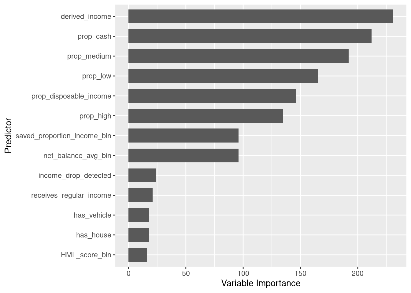
Having a look at predictors in the Affluency category for Retailer R2 General Merchandise Spend it can be seen that derived income is the most important predictor when establishing whether a customer shops at our stores or at our competitors. This variable is ranked the 4th most important across all predictors. The average derived income for our customers is R24,261 while the average derived income at our competitors is R30,874. This tells us that customers spending at our competitors are earning a higher income on average.

data <- readRDS(file = '../../static/data/MyComp_Cust_variable_importance_record.RDS')
plot_data <- data %>% filter(Retailer == 'R2' & Category == 'General M' & pred_category == 'Affluency')

p <- ggplot(plot_data, aes(x = reorder(variable_name, variable_importance), y = variable_importance)) +
  geom_col( width = 0.7) + coord_flip() + ylab("Variable Importance") + xlab("Predictor")
p

StatsLab