Data Wrangling
Why data-wrangling
If you can wrangle data into the proper form you can do anything with it…

Data-wrangling is absolutely essential for every data science task where we need to work with collected data.
A recent article from the New York Times said “Data scientists, according to interviews and expert estimates, spend from 50 percent to 80 percent of their time mired in the mundane labor of collecting and preparing data, before it can be explored for useful information.”
An excelent talk on data wrangling by Jenny Bryan:
https://www.youtube.com/watch?v=4MfUCX_KpdE
It is important to highlight the following facts;
- Excellent data wrangling skills will allow you to make R tools “flow” into one another.
- Different functions require different input formats and so do different solutions!
- The correct shape for the data will greatly simplify the stats needed to solve a problem.
- For example where you would have looped over data you can now simply aggregate
- For example where you would have repeated a model or visualization you now apply it over a hierarchy!
- Being data fluent will allow you to come up with innovative solutions!
The basics - tabular data examples
Here we will use an example of grocery store data.
Import data
What does the data look like?:
dummy_data <-
  readRDS("../../static/data/data-wrangling/dummy_data.rds")

dummy_data %>% glimpse
## Observations: 1,000
## Variables: 10
## $ customer_no <chr> "49ef700455a56debe3214598663330f6", "210d4179edb2...
## $ spend_month <dttm> 2012-12-01, 2012-12-01, 2012-12-01, 2012-12-01, ...
## $ store_counts <int> 1, 1, 1, 1, 1, 1, 1, 1, 1, 1, 1, 1, 1, 1, 1, 1, 1...
## $ visits_count <int> 1, 1, 1, 1, 1, 1, 1, 1, 1, 1, 1, 1, 2, 1, 1, 1, 1...
## $ item_sum <int> 1, NA, 6, 4, 1, 1, 1, NA, 4, 1, 1, 1, 1, 1, NA, 2...
## $ discount_sum <dbl> 0.00, 0.00, 4.05, 0.00, 0.00, 6.90, NA, 0.00, 10....
## $ spend_sum <dbl> 40.00, 15.90, 41.90, 117.96, NA, 43.25, 31.90, 18...
## $ spend_day <chr> "Fri", "Wed", "Wed", "Sun", "Fri", "Wed", "Wed", ...
## $ spend_time <chr> "afternoon", "afternoon", "evening", "lunch", "ev...
## $ spend_type <chr> "protein", "non_cash", "prepared_and_deli", "dair...Reshaping to answer a question
The basics
Widening
What if I asked you; “Show me the spend in each spend_time on a customer level”.
For a person and also for some models you will need to widen the data. By ‘widen’ we mean adding columns. Humans read better when you describe an obeservation using columns after all…
To widen this data we use the function tidyr::spread
dummy_data %>%
  select(customer_no,spend_time,spend_sum) %>%
  tidyr::spread(key = spend_time, value = spend_sum, fill = 0)
## # A tibble: 998 x 6
## customer_no afternoon evening lunch morning `<NA>`
## <chr> <dbl> <dbl> <dbl> <dbl> <dbl>
## 1 001dc4f17ad2f7999c215ac147ad9a13 0 0 0 93.0 0
## 2 0020cab9597c12589249daa13a1427a8 30.8 0 0 0 0
## 3 0068525ef1d0d392ad3e97602511551a 59.9 0 0 0 0
## 4 00d75bffda7ea469a511c891a28b2df2 0 0 25.0 0 0
## 5 011aec649b655991c2835f151188c54e 0 0 0 0 0
## 6 014dd528202b032a46564f63100ced5c 0 0 0 422 0
## 7 015392d5b1b6e0b63a4ca5ce1139d4ac 0 30.0 0 0 0
## 8 01948501615939ecb5a8c49af2ab45dd 0 0 0 13.0 0
## 9 01a86d2dba1514e5a92ecb38b408bbe8 43.8 0 0 0 0
## 10 0210fe573d0e13b2cd68cabe31d3a94c 0 0 7.90 0 0
## # ... with 988 more rowsWhat were the averages for these metrics?
wide_summarised <-
  dummy_data %>%
  select(customer_no,spend_time,spend_sum) %>%
  tidyr::spread(key = spend_time, value = spend_sum, fill = 0) %>%
  summarise_if(is.numeric,mean,na.rm=TRUE)

wide_summarised
## # A tibble: 1 x 5
## afternoon evening lunch morning `<NA>`
## <dbl> <dbl> <dbl> <dbl> <dbl>
## 1 19.8 13.5 21.1 20.9 0.271Moving back to long format
This was very basic, but what if we wanted to do this in reverse?
Of course we can do the exact opposite using tidyr::gather
Let’s visualize the spend in each time category by moving back to the less natural ‘long’ format. Functions generally become more powerful the longer we can shape the data since they naturally scan vectors of columns
wide_summarised %>%
  tidyr::gather(key = "time_category", value = "average_spend") %>%
  ggplot(aes( x = time_category, y = average_spend))+
  geom_bar(stat = "identity")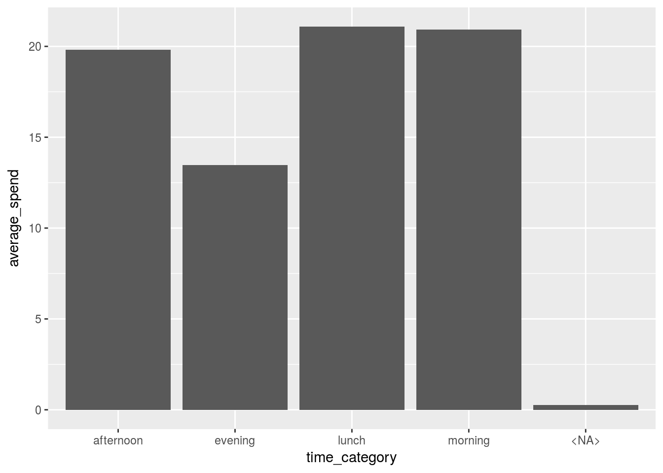
With the wide format we would need to plot each column individually but now we can do them altogether.
Bit of both
What if I asked you “Show me all the time interactions for numeric variables on a customer level”
Let’s look at the releavant data for spend again:
dummy_data %>%
  select_if(is.numeric)
## # A tibble: 1,000 x 5
## store_counts visits_count item_sum discount_sum spend_sum
## <int> <int> <int> <dbl> <dbl>
## 1 1 1 1 0 40.0
## 2 1 1 NA 0 15.9
## 3 1 1 6 4.05 41.9
## 4 1 1 4 0 118
## 5 1 1 1 0 NA
## 6 1 1 1 6.90 43.2
## 7 1 1 1 NA 31.9
## 8 1 1 NA 0 186
## 9 1 1 4 10.0 14.0
## 10 1 1 1 NA 15.0
## # ... with 990 more rowsHow would I wrangle out the interactions?
Well one way is to name the interactions by gathering the relevant metrics together before we widen them
dummy_data %>%
  select(store_counts,item_sum,discount_sum,spend_sum,customer_no,spend_time) %>%
  gather(key = "metric", value = "value",-customer_no, -spend_time) %>%
  mutate(interaction = paste0(spend_time,"_",metric)) %>%
  spread(key = interaction,value = value)
## # A tibble: 4,000 x 23
## customer_no spend_time metric afternoon_discou… afternoon_item_…
## <chr> <chr> <chr> <dbl> <dbl>
## 1 001dc4f17ad2f79… morning discoun… NA NA
## 2 001dc4f17ad2f79… morning item_sum NA NA
## 3 001dc4f17ad2f79… morning spend_s… NA NA
## 4 001dc4f17ad2f79… morning store_c… NA NA
## 5 0020cab9597c125… afternoon discoun… 15.0 NA
## 6 0020cab9597c125… afternoon item_sum NA 3.00
## 7 0020cab9597c125… afternoon spend_s… NA NA
## 8 0020cab9597c125… afternoon store_c… NA NA
## 9 0068525ef1d0d39… afternoon discoun… NA NA
## 10 0068525ef1d0d39… afternoon item_sum NA 5.00
## # ... with 3,990 more rows, and 18 more variables:
## # afternoon_spend_sum <dbl>, afternoon_store_counts <dbl>,
## # evening_discount_sum <dbl>, evening_item_sum <dbl>,
## # evening_spend_sum <dbl>, evening_store_counts <dbl>,
## # lunch_discount_sum <dbl>, lunch_item_sum <dbl>, lunch_spend_sum <dbl>,
## # lunch_store_counts <dbl>, morning_discount_sum <dbl>,
## # morning_item_sum <dbl>, morning_spend_sum <dbl>,
## # morning_store_counts <dbl>, NA_discount_sum <dbl>, NA_item_sum <dbl>,
## # NA_spend_sum <dbl>, NA_store_counts <dbl> # arrange(-afternoon_spend_sum)Changing a problem
Let’s say for instance we have the following data:
dummy_data_2 <-
tibble(shop = LETTERS,
       churn_rate = runif(26, 0, 1),
       attrition = runif(26, 0, 1),
       join_rate = runif(26, 0, 1),
       sales = rnorm(1,mean = 5, sd = 3)*runif(26,10^2,10^4))

dummy_data_2
## # A tibble: 26 x 5
## shop churn_rate attrition join_rate sales
## <chr> <dbl> <dbl> <dbl> <dbl>
## 1 A 0.986 0.506 0.447 3409
## 2 B 0.588 0.0882 0.637 42124
## 3 C 0.804 0.0999 0.0627 9262
## 4 D 0.233 0.192 0.469 35910
## 5 E 0.0441 0.292 0.0621 13394
## 6 F 0.0300 0.675 0.656 32413
## 7 G 0.991 0.152 0.826 20847
## 8 H 0.141 0.895 0.395 51524
## 9 I 0.970 0.220 0.00620 9599
## 10 J 0.834 0.587 0.182 4008
## # ... with 16 more rowsIf we wanted to take the each shop row and multiply the columns together to find the multiplicative affect how would we do it?
One way to do this is to use some form of apply function:
dummy_data_2 %>%
  select(-1) %>%
  apply(function(x) prod(x),MARGIN = 1)
## [1] 758.97678 1391.16293 46.65377 755.62063 10.71378
## [6] 430.42521 2589.78481 2566.70058 12.69749 357.94699
## [11] 11380.89775 2404.21539 7869.61525 141.64731 364.92837
## [16] 14655.70645 517.01111 1075.52391 2197.33395 120.62184
## [21] 246.22134 120.96861 42.18102 2226.17664 43.17457
## [26] 5226.73185This feels sort of ugly and returns a vector… We would prefer to remain type stable here inside a dataframe.
We could simply reshape this data so that we are infact summarizing over rows not columns:
dummy_data_2 %>%
  gather(key = "metric", value = "value",-shop) %>%
  group_by(shop) %>%
  summarise(prod = value %>% prod)
## # A tibble: 26 x 2
## shop prod
## <chr> <dbl>
## 1 A 759
## 2 B 1391
## 3 C 46.7
## 4 D 756
## 5 E 10.7
## 6 F 430
## 7 G 2590
## 8 H 2567
## 9 I 12.7
## 10 J 358
## # ... with 16 more rowsBy reshaping the data we remain inside of a tidy context while leveraging our sql like backend dplyr to solve the problem
Advanced wrangling
How do we use wrangling when the data and the question become more complex?
Let’s follow through the examples given by Jenny Brian on the Game Of Thrones data
About the data
Here we have a dataset api that we can use to pull data out about any Game Of Thrones character.
The api can be found via:
https://anapioficeandfire.come
Let’s look at what we get if we ask for some jason data on all the characters (1 entry):
data_characters_request <-
  # httr::GET(url = "https://anapioficeandfire.com/api/characters?pageSize=1000")
  httr::GET(url = "https://www.anapioficeandfire.com/api/characters")

data_characters <-
  data_characters_request %>%
  content()


data_characters[[1]]
## $url
## [1] "https://www.anapioficeandfire.com/api/characters/1"
##
## $name
## [1] ""
##
## $gender
## [1] "Female"
##
## $culture
## [1] "Braavosi"
##
## $born
## [1] ""
##
## $died
## [1] ""
##
## $titles
## $titles[[1]]
## [1] ""
##
##
## $aliases
## $aliases[[1]]
## [1] "The Daughter of the Dusk"
##
##
## $father
## [1] ""
##
## $mother
## [1] ""
##
## $spouse
## [1] ""
##
## $allegiances
## list()
##
## $books
## $books[[1]]
## [1] "https://www.anapioficeandfire.com/api/books/5"
##
##
## $povBooks
## list()
##
## $tvSeries
## $tvSeries[[1]]
## [1] ""
##
##
## $playedBy
## $playedBy[[1]]
## [1] ""What info did we recieve from the api?
data_characters[[1]] %>% names## [1] "url" "name" "gender" "culture" "born"
## [6] "died" "titles" "aliases" "father" "mother"
## [11] "spouse" "allegiances" "books" "povBooks" "tvSeries"
## [16] "playedBy"Let’s get all the data from the api:
extract_api_data <- function(page = 1) {

  data_characters_request <-
  httr::GET(url = paste0("https://anapioficeandfire.com/api/characters?page=",page)) %>%
    content()

}

all_pages <-
  map(1:214,extract_api_data)

all_pages %>%
  saveRDS("../../static/data/data-wrangling/all_pages.rds")
OK, so we have a nested structure of data describing each GOT character…
Let’s see which characters we have in here…
# data_characters <-
#   all_pages %>%
#   unlist(recursive = FALSE)

data_characters %>%
  map("name") %>%
  tail(20)
## [[1]]
## [1] "Wyl"
##
## [[2]]
## [1] "Wyl"
##
## [[3]]
## [1] "Wylla"
##
## [[4]]
## [1] "Xaro Xhoan Daxos"
##
## [[5]]
## [1] "Xhondo"
##
## [[6]]
## [1] "Yandry"
##
## [[7]]
## [1] "Ygon"
##
## [[8]]
## [1] "Ygritte"
##
## [[9]]
## [1] "Yna"
##
## [[10]]
## [1] "Yorkel"
##
## [[11]]
## [1] "Yorko Terys"
##
## [[12]]
## [1] "Yormwell"
##
## [[13]]
## [1] "Young Henly"
##
## [[14]]
## [1] "Ysilla"
##
## [[15]]
## [1] "Zarabelo"
##
## [[16]]
## [1] "Zei"
##
## [[17]]
## [1] "Zekko"
##
## [[18]]
## [1] "Zharaq zo Loraq"
##
## [[19]]
## [1] "Zollo"
##
## [[20]]
## [1] "Criston Cole"Put this into a dataframe:
GOT_df <-
  map_df(data_characters,`[`, c("name","gender","culture","born","died")) %>%
    mutate(titles = data_characters %>% map("titles"))

GOT_df %>% sample_n(20)
## # A tibble: 20 x 6
## name gender culture born died titles
## <chr> <chr> <chr> <chr> <chr> <list>
## 1 Mezzara Female Ghiscari At Meereen "" <list …
## 2 Daeron Targaryen Male "" In 114 AC In 130 AC, a… <list …
## 3 Dake Male "" "" At Coldmoat <list …
## 4 Robin Hill Male "" "" "" <list …
## 5 Steffon Swyft Male "" "" "" <list …
## 6 Tyrion Tanner Male "" In 300 AC, at … "" <list …
## 7 Drennan Male Ironborn "" In 299 AC, a… <list …
## 8 Dacey Mormont Female Northmen In or between … In 299 AC, a… <list …
## 9 Wat Male "" "" "" <list …
## 10 Agrivane Male "" "" "" <list …
## 11 Jeyne Swann Female "" "" "" <list …
## 12 Bronn Male "" In or between … "" <list …
## 13 Tregar Male "" "" In 298 AC, a… <list …
## 14 Luthor Tyrell Male "" "" "" <list …
## 15 Layna Female "" In or between … "" <list …
## 16 Edwyd Fossoway Male "" "" In 299 AC, a… <list …
## 17 Elys Westerling Male "" "" "" <list …
## 18 Kyleg Male Free Folk "" "" <list …
## 19 Aggo Male Dothraki "" "" <list …
## 20 Sarra Frey Female "" In 285 AC "" <list …So we can pull out the data from these nested lists into other columns or even apply models to them…
Let’s visualize the cultures of all the characters:
GOT_df %>%
  filter(culture != "") %>%
  # select(-data_char) %>%
  ggplot()+
  geom_bar(aes(x = culture, y = ..count.., fill = culture))+
  ggplot2::theme(axis.text.x = element_text(angle = 90, hjust = 1))+
  coord_flip()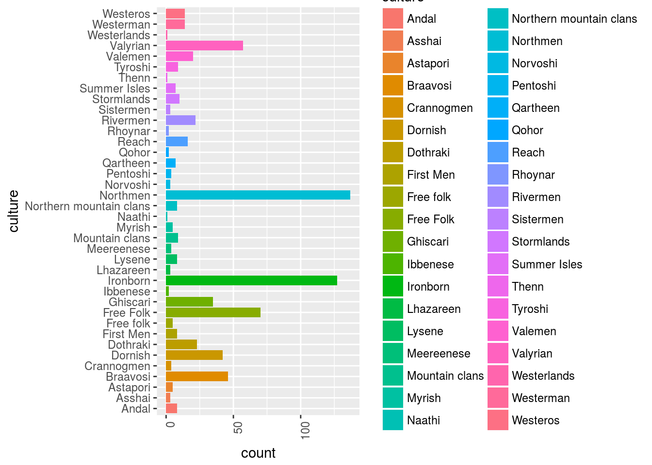
OK, so in this sample sent back from the api we have this distribution of characters by cultures.
How many people died?
GOT_df %>%
  filter(culture != "") %>%
  mutate(died = ifelse(died == "",0,1)) %>%
  # select(-data_char) %>%
  ggplot()+
  geom_bar(aes(y = died, x = culture, fill = culture), stat = "identity")+
  ggplot2::theme(axis.text.x = element_text(angle = 90, hjust = 1))+
  coord_flip()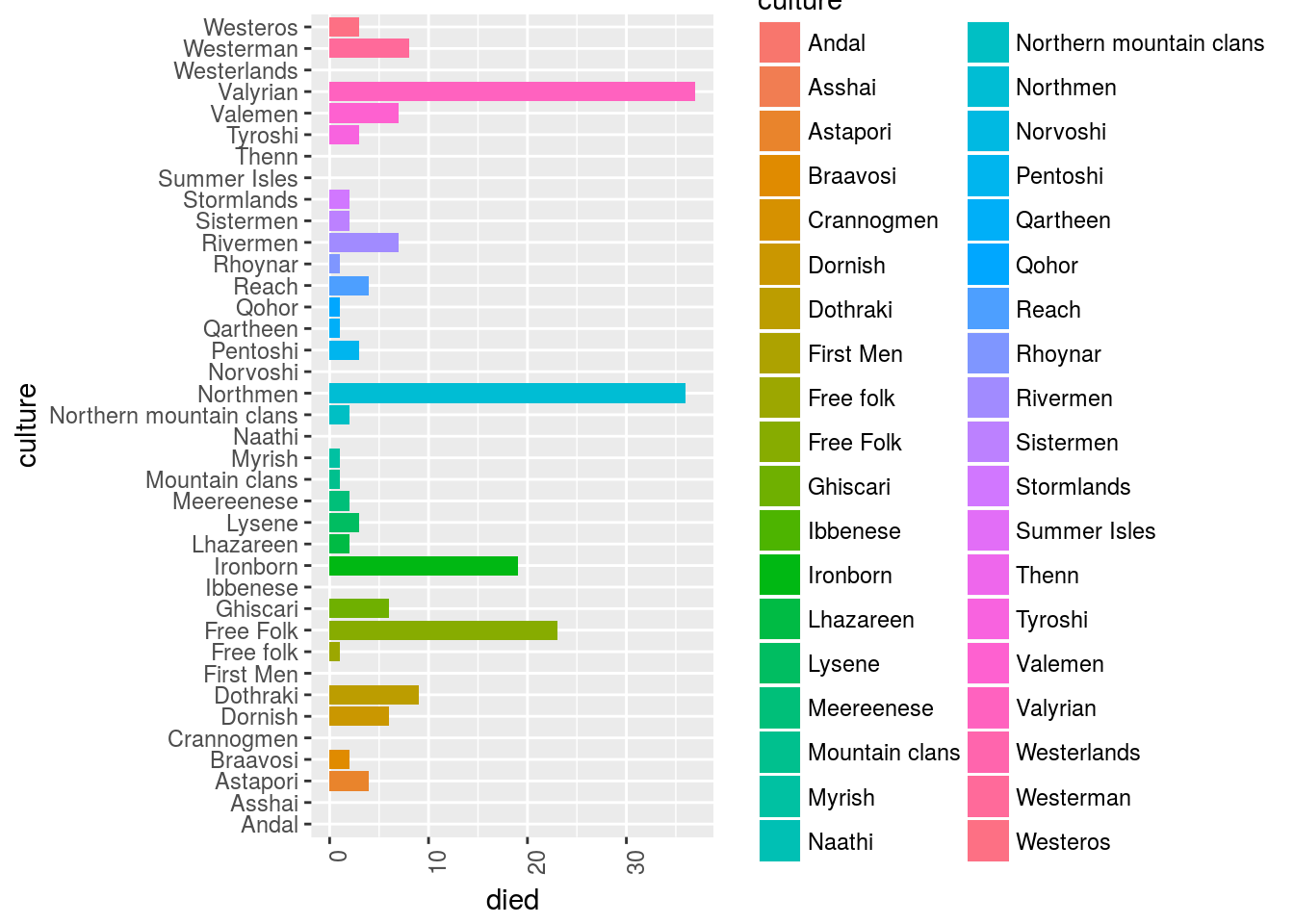
What’s the probability of dying if you have some sort of title:
GOT_df %>%
  mutate(died = ifelse(died == "",FALSE,TRUE)) %>%
  mutate(has_title = titles %>% map_lgl(~ifelse(any(.x != ""), TRUE, FALSE))) %>%
  group_by(has_title,died) %>%
  tally %>%
  spread(key = died, value = n, sep = "_") %>%
  mutate(prob_of_dying = died_TRUE/(died_TRUE+died_FALSE))
## # A tibble: 2 x 4
## # Groups: has_title [2]
## has_title died_FALSE died_TRUE prob_of_dying
## <lgl> <int> <int> <dbl>
## 1 F 797 251 0.240
## 2 T 784 302 0.278