Automated parameter selection for LOESS regression

Typically, when we want to understand the relationship between two variables we simply regress one on the other, plot the points and fit a linear trend line. To illustrate this, we use the EuStockMarkets datset pre-loaded in R. The data-set contains the daily closing prices of major European stock indices. We will focus on the FTSE. Below, we regress the FTSE daily closing price data on time (what we will call an “Index”) and plot a linear trend. I use the stats package to execute the regressions and the ggplot2 package to generate the plots. I also use the fANCOVA package, but more about this later. As we expect, we see a clear linear trend over time.

library(stats,quietly = T)
library(ggplot2,quietly = T)
library(fANCOVA,quietly = T)

## fANCOVA 0.5-1 loaded

FTSE_close <- EuStockMarkets[,4]
Index <- seq(1, length(FTSE_close), by = 1)
FTSE.lm <- lm(FTSE_close ~ Index, data = EuStockMarkets)
FTSE.lm.predict <- predict(FTSE.lm,  data.frame(Index=Index))

## Don't know how to automatically pick scale for object of type ts. Defaulting to continuous.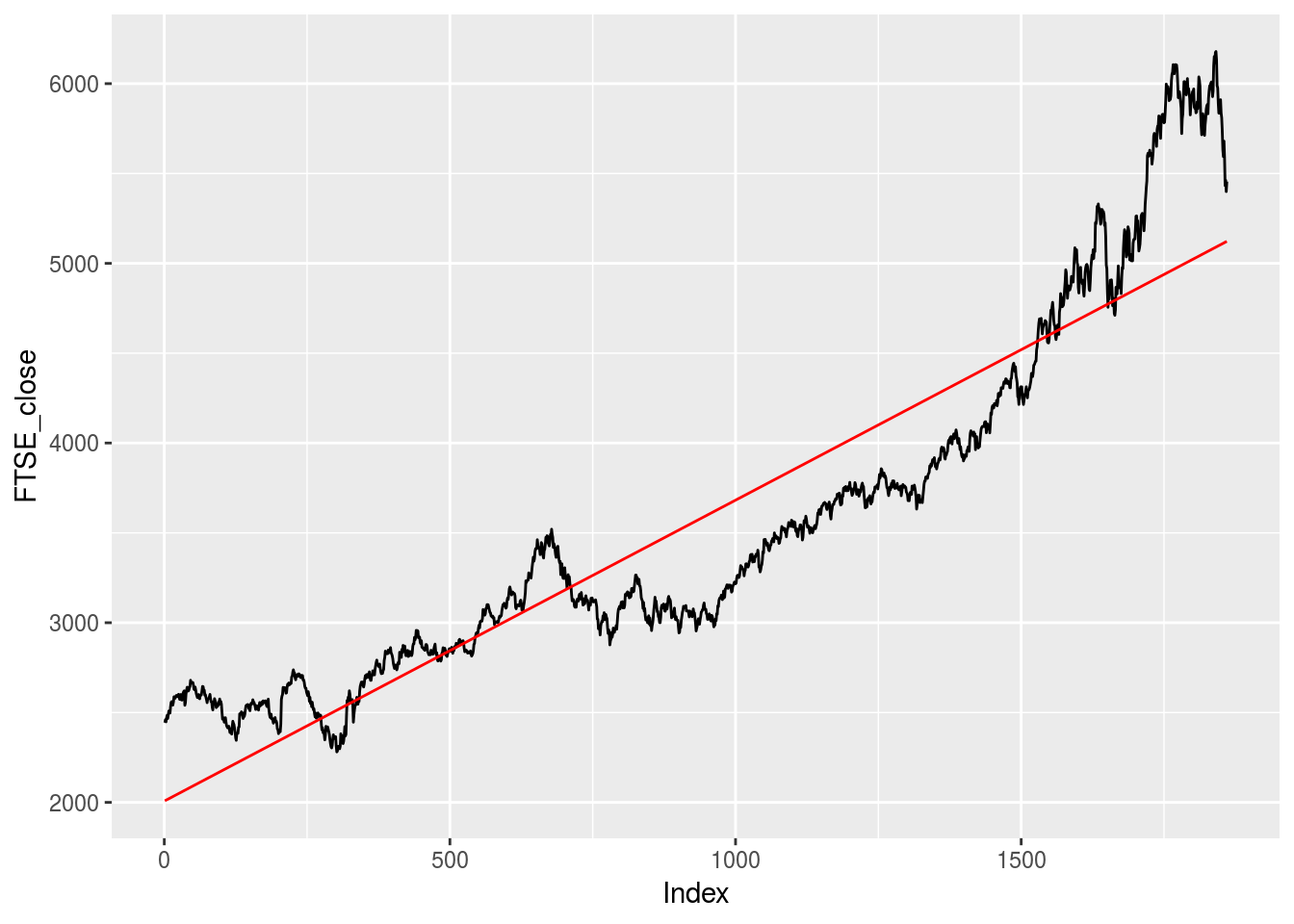

In some cases however, one may want a non-linear trend line that reflects the movement in the data. One way to obtain this would involve a LOESS/LOWESS regression. A LOESS/LOWESS (Locally Weighted Scatter-plot Smoother) regression involves fitting a smooth curve between two or more points in a series. A LOESS regression allows one to regress up to four covariates on an outcome variable and divides the data at hand into localized subsets and fits regressions on each of these subsets. After obtaining the LOESS regression results, a LOESS curve can be fitted through the data series where each point is obtained by weighting the different regressions. Below we plot a typical LOESS curve on our FTSE closing prices.

FTSE.lo <- loess(FTSE_close ~ Index, data = EuStockMarkets)
FTSE.lo.predict <- predict(FTSE.lo, data.frame(Index=Index), span = 0.3)

## Don't know how to automatically pick scale for object of type ts. Defaulting to continuous.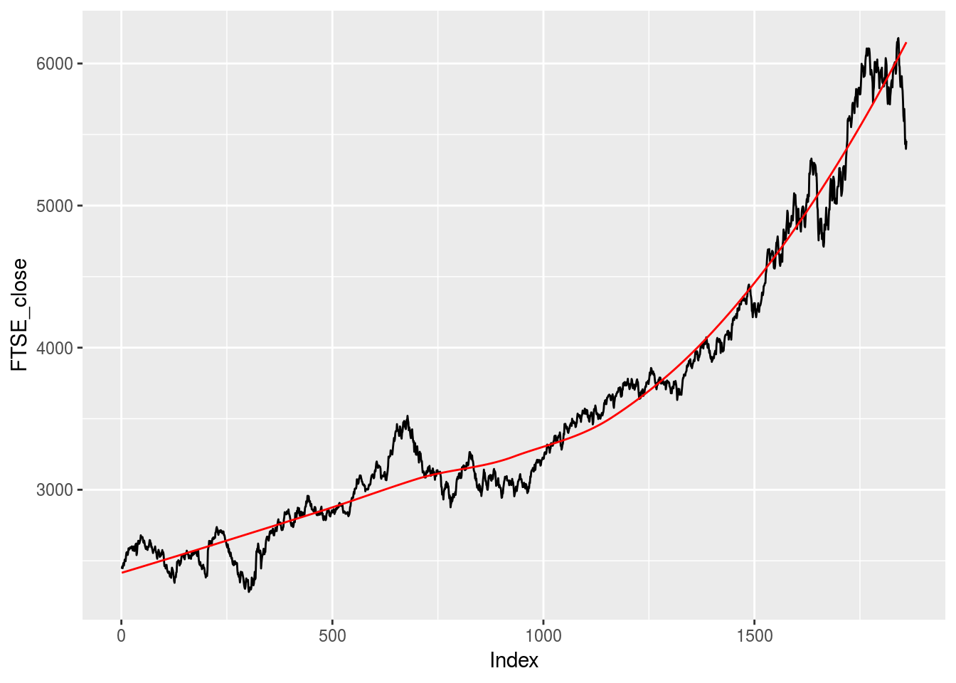

As can be seen, the LOESS curve creates a much smoother trend line through the data than a simple linear trend. However, unlike the linear prediction, the LOESS prediction involves another parameter, namely span. This parameter controls how the fit at a specific point in the series weights the data nearest to it. If this parameter is set too large, the regression will be over-smoothed while setting a span too small will result in large variance given that there will be insufficient data near a point to ensure an accurate point. To see this, below we plot a LOESS curve with a span of 0.1 and a span of 0.9.

FTSE.lo1 <- loess(FTSE_close ~ Index, data = EuStockMarkets, span = 0.1)
FTSE.lo.predict1 <- predict(FTSE.lo1, data.frame(Index=Index))
FTSE.lo2 <- loess(FTSE_close ~ Index, data = EuStockMarkets, span = 0.9)
FTSE.lo.predict2 <- predict(FTSE.lo2, data.frame(Index=Index))

## Don't know how to automatically pick scale for object of type ts. Defaulting to continuous.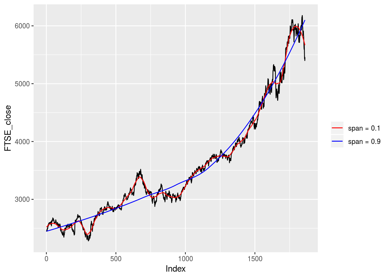

As can be seen, setting the span to 0.1 leads to over-fitting, i.e. the LOESS curve resembles the series too closely, while setting the span to 0.9 leads to under-fitting, i.e. the LOESS curve provides little information. Typically, one would fit numerous LOESS curves with various span values and graphically decide which span value results in the desired fit. While such a visual approach is intuitive, it lacks robustness. In this sense, one would prefer to choose a span value that optimizes the fit of the LOESS curve. I recently came across the loess.as function in the fANCOVA package, see https://cran.r-project.org/web/packages/fANCOVA/index.html. This function fits a LOESS regression and automates the parameter selection process. In selecting the optimal span value, it gives the option of either a bias-corrected Akaike information criterion (AICC) method or a Generalized Cross-Validation (GCV) method. Below we run this LOESS regression, choosing the GCV option, and plot the LOESS curve.

FTSE.lo3 <- loess.as(Index, FTSE_close, degree = 1, criterion = c("aicc", "gcv")[2], user.span = NULL, plot = F)
FTSE.lo.predict3 <- predict(FTSE.lo3, data.frame(Index=Index))

## Don't know how to automatically pick scale for object of type ts. Defaulting to continuous.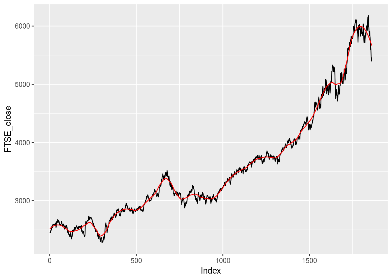

It is however important to note that the choice of parameter selection method, AICC vs GCV, tends to provide rather different span values. In this case, it’s best to take time and understand the characteristics of your data and the nature of your task at hand before choosing a method. The loess.as function also has a few other parameters which can be adjusted, such as the degree of polynomials to be used. Go ahead and toy around with these to find what works best for your application.

In short, While I will still probably revert to plotting various LOESS curves and comparing the fits graphically, this package allows me to test my intuitive choice of a span value against a more robust value, which I think is pretty useful.