
A Survey of Uplift at 8020
Introduction
In consumer analytics it is very important to measure the effectiveness of your marketing and campaign management.

Unfortunately each company may have a different oppertunity-infrastructure proposition. Some may run product campaigns. Others run loyalty programs for customers. Some programs have already been run or outbound communication has already been sent out before it was decided to run performance analytics.

All of these variations make measuring uplift quite complicated. In particular different teams on different projects will have significantly different strategies for measuring uplift.
The purpose of this blog post is to collate information on the different uplift methodologies employed and the use cases for those. Some suggestions and recommendations are also made regarding the different methodologies.
How is uplift measured
In broad terms uplift can be measured following the following strategy:
- Estimate response for a control group.
- Calculate expected response for test group.
- Calculate lift of actual response over expected response.
When modelling this can be done on a person basis because we can predict the desired response using the replicant covariates.
For a given response \(Y_i\) as the take up or conversion of a customer say we can define uplift mathematically:
\(E(Y_i | X_i) = f(T_i,X_i,T_i * X_i) = E(Y_i | X_i, T_i = 1) - E(Y_i | X_i, T_i = 0)\)
Both predictions can be made using a trained model by setting the treatment indicator $ T_i $ and predicting the outcome for that row.
This is very similar to the group calculation in the steps above. We are comparing the expected outcome given a control with what actually happened. Although in the model case you can also use the expected value for the treated case.
Uplift measurement vs A/B testing
When we haven’t run our campaign or targeted outbound advertising we can setup a DoE in advance. We can then do simple A/B testing to determine which campaigns are the best and even make some causal inference.
For general uplift measurement we don’t need to be this precise or a DoE may cost too much time or money. Additionally we may already have outbound advertisement or measured the response.
Uplift measurement doesn’t try to make any causal inference. We are only interested in measuring the treatment effect due to having been treated.
DOE
If you want to look at my blog on the basics of DoE in R go look at:
https://statslab.eighty20.co.za/posts/design_and_analysis_of_experiments_with_r/
Matching
When treatment is already observed in the absence of a DoE or control group you may want to consider matching.
The idea behind DoE is constructing treatment groups such that condounding factors are randomized over the control groups.
This way we control for the contribution of factors that are not of interest.
With matching we pair up each response with a doppelganger. If we assign the new balanced groups of treated and matched as if the matched was the control group we cater for confounding variables since the groups are statistically similar.
Careful! You can only control for variables you are matching on!
Matching methods
- Simple propensity matching
A model is fit predicting the response. This yields a propensity when predicted for each response.
Care is taken that the distribution of the propensity is smooth. Then we match responses based on their propensity score.
- Genetic matching
Genetic algorithms are very good at solving optimization problems in a robust way. This approach is unfortunately very resource/time expensive.
This method will avoid matching individuals with similar propensity scores but different features (different reasons for having the same propensity).
This feature is very attractive when you want to control for lurker effects. Although from a statistical point of view the propensity matching may be balanced in aggregate (i.e. if by response uplift is not important).
- Random forest matching
Here we fit a random forest predicting the response. Make sure to store the terminal nodes! Once our model is trained we can use the proximity matrices for responses to match entries that often end up in the same terminal leaves.
Unlike 1D matching the members are similar based on partitioning of variables. This way different people won’t end up with similar distance/entropy scores and get matched.
What is considered lift
When measuring take up or conversion rates we define 4 general responses:
- The Persuadables : customers who only respond to the marketing action because they were targeted
- The Sure Things: customers who would have responded whether they were targeted or not
- The Lost Causes: customers who will not respond irrespective of whether or not they are targeted
- The Do Not Disturbs or Sleeping Dogs : customers who are less likely to respond because they were targeted
We can illustrate this using:
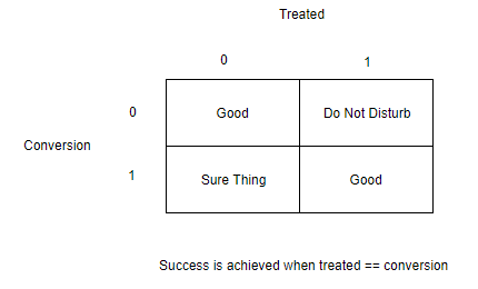
We do not want to measure lift on cases where they would have converted anyway. We also wouldn’t want to target people who will respond negatively.
Methodologies and use cases
Campaign analytics
Some campaign performance analytics were performed for a large FMCG retailer on their in-store campaigns. These campaigns did not have any outbound advertising or targeting. All adverts were shown instore only and discounts were given at point of sale.
Analysis was performed post response ons selected stores and brands.
It was decided that uplift would be measured on a basket level to estimate how much the campaign has pushed instore basket value.
A Pre-Post measurement methodology was decided. To overcome some of the drawbacks of this approach a control group was established. Baskets were identified based on qualifying criteria like the tender type for payment method.
A design matrix was setup for each day over the campaign period starting with a pre-period. Using a GLS model the basket value was predicted over the period of the campaign for both groups.
By further predicting the treatment group assuming no treatment uolift was measured using this counter factual.
Basic membership benefit analysis
Product benefit analysis was measured for a large bank using established control groups to measure the benefit offering these products to companies
A GLM was fit on the data predicting the revenue response of interest. Using the trained model the expected effect size was estimated for applying the treatment to each business.
FMCG loyalty analysis within their healthy foods department
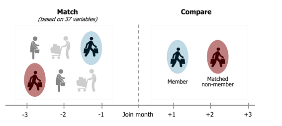
In this case we had already measured the take up of membership of the program and we had no measurement of targeted or treatment groups.
In this case we could assume the response of interest is total spend per customer on healthy foods and that the treatment is giving this person membership to the program. This has some issues due to likely lurker effects. With no randomization and the fact that the treatment is self selected we would have no control over the biases in this treatment variable.
To address this genetic matching was performed, matching customers who have recorded take up of membership to others who have not. By matching a person onto a doppelganger we attempt to control for confounding effects in the analysis.
Without even predicting the expected treatment effect for members we could compare each person to his doppelganger and report a lift of spend over the periods following the join date for each member.
Matches were made on the last quarter of data leading into the month of joining the program.